Example 1: Turing patterns in 2D reaction-diffusion#
In this case, we consider a simple 2D geometry comprised of two compartments:
surf - 2D surface
edge - outer edges of the surface (1D)
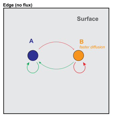
We implement the Schnakenberg model as a simple system that exhibits Turing patterns in 2D. In this model, two species diffuse in a single compartment (“surf”), A and B. A is produced autocatalytically and inhibits the production of B. B degrades over time and positively regulates the production of A.
from matplotlib import pyplot as plt
import matplotlib.image as mpimg
img_A = mpimg.imread('schnakenberg-diagram.png')
plt.imshow(img_A)
plt.axis('off')
(-0.5, 3760.5, 3782.5, -0.5)
Nondimensionalizing, with \(\bar{A}=A/c_{ref}\) and \(\bar{B}=B/c_{ref}\), the Schnakenberg model is typically written in the form:
where \(a\) and \(b\) are reaction constants, \(\gamma\) is a scaling factor, and \(d\) is the ratio of the two diffusion coefficients (\(D_B/D_A\)). One requirement for forming Turing patterns is that \(D_B > D_A\), so \(d\) must be greater than 1 (here, we set it equal to 20).
To define the system below, we recover the dimensional form of these equations (SMART requires a form with dimensions):
where \(\gamma^* = \gamma D_A / L^2\).
We solve these equations over a 1 by 1 square domain with no-flux boundary conditions.
We begin with the necessary imports:
import dolfin as d
import sympy as sym
import numpy as np
import pathlib
import gmsh  # must be imported before pyvista if dolfin is imported first

from smart import config, common, mesh, model, mesh_tools, visualization
from smart.units import unit
from smart.model_assembly import (
    Compartment,
    Parameter,
    Reaction,
    Species,
    SpeciesContainer,
    ParameterContainer,
    CompartmentContainer,
    ReactionContainer,
)
import logging
/usr/lib/python3/dist-packages/scipy/__init__.py:146: UserWarning: A NumPy version >=1.17.3 and <1.25.0 is required for this version of SciPy (detected version 1.26.4
  warnings.warn(f"A NumPy version >={np_minversion} and <{np_maxversion}"
We will set the logging level to INFO. This will display some output during the simulation. If you want to get even more output you could set the logging level to DEBUG.
logger = logging.getLogger("smart")
logger.setLevel(logging.INFO)
Futhermore, you could also save the logs to a file by attaching a file handler to the logger as follows.
file_handler = logging.FileHandler("filename.log")
file_handler.setFormatter(logging.Formatter(smart.config.base_format))
logger.addHandler(file_handler)
We define the various units for use in the model.
# Aliases - base units
um = unit.um
molecule = unit.molecule
sec = unit.sec
dimensionless = unit.dimensionless
D_unit = um**2 / sec
flux_unit = molecule / (um * sec)
surf_unit = molecule / um**2
edge_unit = molecule / um
Generate model#
Compartments#
As described above, the two compartments are the “surf” (2D) and edge (1D). These are initialized by calling:
compartment_var = Compartment(name, dimensionality, compartment_units, cell_marker)
where
name: string naming the compartment
dimensionality: topological dimensionality (e.g. 2 for surf, 1 for edge)
compartment_units: length units for the compartment (um for both here)
cell_marker: integer marker value identifying each compartment in the parent mesh
surf = Compartment("surf", 2, um, 1)
edge = Compartment("edge", 1, um, 3)
Now we initialize a compartment container and add both compartments to it.
cc = CompartmentContainer()
cc.add([surf, edge])
Species#
In this case, we have a two species, “A” and “B”, which exist in the 2D “surf” domain. Each is initialized by calling:
species_var = Species(
            name, initial_condition, concentration_units,
            D, diffusion_units, compartment_name, group (opt)
        )
where
name: string naming the species
initial_condition: initial concentration for this species (can be an expression given by a string to be parsed by sympy - the only unknowns in the expression should be x, y, and z)
concentration_units: concentration units for this species (molecules/μm2 here)
D: diffusion coefficient
diffusion_units: units for diffusion coefficient (μm2/sec here)
compartment_name: each species should be assigned to a single compartment (“surf”, here)
group (opt): for larger models, specifies a group of species this belongs to; for organizational purposes when there are multiple reaction modules
Note that in this example, we initially define some other constants to convert from the nondimensional formulation to dimensional equations.
D_A = 0.0001  # diffusion coefficient of species A
d_ratio = 20.0  # ratio between diffusion coefficients
L = 1.0  # typical length scale for nondimensionalization
a_val = 0.1
b_val = 1
Ainit = a_val + b_val
Binit = b_val / (a_val + b_val)**2
A = Species("A", Ainit, surf_unit, D_A, D_unit, "surf")  # activator
B = Species("B", Binit, surf_unit, d_ratio*D_A, D_unit, "surf")  # inhibitor
Create a species container and add both species to it:
sc = SpeciesContainer()
sc.add([A, B])
Parameters and Reactions#
Parameters and reactions are generally defined together, although the order does not strictly matter. Parameters are specified as:
param_var = Parameter(name, value, unit, group (opt), notes (opt), use_preintegration (opt))
where
name: string naming the parameter
value: value of the given parameter
unit: units associated with given value
group (optional): optional string placing this reaction in a reaction group; for organizational purposes when there are multiple reaction modules
notes (optional): string related to this parameter
use_preintegration (optional): in the case of a time-dependent parameter, uses preintegration in the solution process
Reactions are specified by a variable number of arguments (arguments are indicated by (opt) are either never required or only required in some cases, for more details see notes below and API documentation):
reaction_var = Reaction(
                name, lhs, rhs, param_map,
                eqn_f_str (opt), eqn_r_str (opt), reaction_type (opt), species_map,
                explicit_restriction_to_domain (opt), group (opt), flux_scaling (opt)
            )
name: string naming the reaction
lhs: list of strings specifying the reactants for this reaction
rhs: list of strings specifying the products for this reaction ***NOTE: the lists “reactants” and “products” determine the stoichiometry of the reaction; for instance, if two A’s react to give one B, the reactants list would be [“A”,”A”], and the products list would be [“B”]
param_map: relationship between the parameters specified in the reaction string and those given in the parameter container. By default, the reaction parameters are “kon” and “koff” when a system obeys simple mass action. If the forward rate is given by a parameter “k1” and the reverse rate is given by “k2”, then param_map = {“on”:”k1”, “off”:”k2”}
eqn_f_str: For systems not obeying simple mass action, this string specifies the forward reaction rate By default, this string is “on*{all reactants multiplied together}”
eqn_r_str: For systems not obeying simple mass action, this string specifies the reverse reaction rate By default, this string is “off*{all products multiplied together}”
reaction_type (opt): either “custom” or “mass_action” (default is “mass_action”) [never a required argument]
species_map: same format as param_map; required if other species not listed in reactants or products appear in the reaction string
explicit_restriction_to_domain: string specifying where the reaction occurs; required if the reaction is not constrained by the reaction string (e.g., if production occurs only at the boundary, as it does here, but the species being produced exists through the entire volume)
group (opt): string placing this reaction in a reaction group; for organizational purposes when there are multiple reaction modules
flux_scaling (opt): in certain cases, a given reactant or product may experience a scaled flux (for instance, if we assume that some of the molecules are immediately sequestered after the reaction); in this case, to signify that this flux should be rescaled, we specify ‘’flux_scaling = {scaled_species: scale_factor}’’, where scaled_species is a string specifying the species to be scaled and scale_factor is a number specifying the rescaling factor
For this system, we do not define any reactions on the boundary (edge). This corresponds to assuming a no-flux boundary condition.
gStar = Parameter("gStar", 10000*D_A/L**2, 1/sec)  # gStar = gamma*D_A/L^2
a = Parameter("a", a_val, dimensionless)
b = Parameter("b", b_val, dimensionless)
cref = Parameter("cref", 1.0, surf_unit)  # to convert from dimensionless forms

# Production of A
r1 = Reaction("r1", [], ["A"],
              param_map={"a": "a", "gStar": "gStar", "cref": "cref"},
              eqn_f_str="cref*gStar*(a + (A/cref)**2 * (B/cref))",
              species_map={"A": "A", "B": "B"})

# Degradation of A
r2 = Reaction("r2", ["A"], [],
              param_map={"gStar": "gStar", "cref": "cref"},
              eqn_f_str="cref*gStar*A/cref",
              species_map={"A": "A"})

# Production of B
r3 = Reaction("r3", [], ["B"],
              param_map={"gStar": "gStar", "b": "b", "cref": "cref"},
              eqn_f_str="cref*gStar*b")

# Degradation of B
r4 = Reaction("r4", ["B"], [],
              param_map={"gStar": "gStar", "cref": "cref"},
              eqn_f_str="cref*gStar* (A/cref)**2 * (B/cref)",
              species_map={"A": "A", "B": "B"})
Create parameter and reaction containers and add in associated objects.
pc = ParameterContainer()
pc.add([a, b, gStar, cref])
rc = ReactionContainer()
rc.add([r1, r2, r3, r4])
Create/load in mesh#
In SMART we have different levels of meshes. Here we create a UnitSquare mesh defined by
which will serve as our parent mesh
For our two domains, we have two associated “child meshes”, which are set by the marker functions mf2 and mf1:
surf: in this case, all cells (triangles) belong to this mesh; here, marked by
mf2 = 1edge: 1D child mesh including all line elements along the edges of the domain; here, marked by
mf1 = 3
Note that the marker values must be chosen to match those given in the compartment definitions above.
# define dimensions of domain
x_size = 1.0 * L
y_size = 1.0 * L
# Create mesh
m = 100
n = int(x_size/y_size)*m
rect_mesh = d.RectangleMesh(d.Point(0.0, 0.0), d.Point(x_size, y_size), n, m)
mf2 = d.MeshFunction("size_t", rect_mesh, 2, 1)
mf1 = d.MeshFunction("size_t", rect_mesh, 1, 0)
for e in d.edges(rect_mesh):
    x_vals = np.zeros(2)
    y_vals = np.zeros(2)
    idx = 0
    for vertex in d.vertices(e):
        x_vals[idx] = vertex.point().array()[0]
        y_vals[idx] = vertex.point().array()[1]
        idx = idx+1
    if np.isclose(np.mean(x_vals), 0.) or np.isclose(np.mean(x_vals), x_size)\
            or np.isclose(np.mean(y_vals), 0.) or np.isclose(np.mean(y_vals), y_size):
        mf1[e] = 3
Now we write mesh and meshfunctions to file and visualize here.
mesh_folder = pathlib.Path("rect_mesh")
mesh_folder.mkdir(exist_ok=True)
mesh_file = mesh_folder / "rect_mesh.h5"
mesh_tools.write_mesh(rect_mesh, mf1, mf2, mesh_file)
visualization.plot_dolfin_mesh(rect_mesh, mf2)
/usr/lib/python3/dist-packages/smart/visualization.py:283: PyVistaDeprecationWarning: This function is deprecated and will be removed in future version of PyVista. Use vtk with osmesa instead.
  pyvista.start_xvfb()
ROOT -2026-03-05 06:56:29,599 trame_server.utils.namespace - INFO - Translator(prefix=None) (namespace.py:65)
ROOT -2026-03-05 06:56:29,645 wslink.backends.aiohttp - INFO - awaiting runner setup (__init__.py:147)
ROOT -2026-03-05 06:56:29,646 wslink.backends.aiohttp - INFO - awaiting site startup (__init__.py:154)
ROOT -2026-03-05 06:56:29,647 wslink.backends.aiohttp - INFO - Print WSLINK_READY_MSG (__init__.py:160)
ROOT -2026-03-05 06:56:29,648 wslink.backends.aiohttp - INFO - Schedule auto shutdown with timeout 0 (__init__.py:166)
ROOT -2026-03-05 06:56:29,648 wslink.backends.aiohttp - INFO - awaiting running future (__init__.py:169)
Finally, we initialize the mesh.ParentMesh object, using the hdf5 file as input.
parent_mesh = mesh.ParentMesh(
    mesh_filename=str(mesh_file),
    mesh_filetype="hdf5",
    name="parent_mesh",
)
2026-03-05 06:56:30,299 smart.mesh - INFO - HDF5 mesh, "parent_mesh", successfully loaded from file: rect_mesh/rect_mesh.h5! (mesh.py:245)
2026-03-05 06:56:30,300 smart.mesh - INFO - 0 subdomains successfully loaded from file: rect_mesh/rect_mesh.h5! (mesh.py:258)
Initialize model and solver#
Now we are ready to set up the model. First we load the default configurations and set the solver config.
config_cur = config.Config()
config_cur.flags.update({"allow_unused_components": True})
config_cur.solver.update(
    {
        "final_t": 50.0,
        "initial_dt": 0.1,
        "time_precision": 6,
    }
)
We create the model object initialize the model using the initialize function found in the smart.model module. We then save the model information to a .pkl file for later reference.
Note that we could later load the model information from the pickle file using the line:
model_cur = model.from_pickle(model_cur.pkl)
model_cur = model.Model(pc, sc, cc, rc, config_cur, parent_mesh)
model_cur.initialize(initialize_solver=False)
model_cur.to_pickle('model_cur.pkl')
2026-03-05 06:56:30,328 smart.model - INFO - Compartment(s), {'edge'}, are unused in any reactions. (model.py:626)
2026-03-05 06:56:30,329 smart.model - INFO - Removing unused compartment(s) from model! (model.py:627)
 2026-03-05 06:56:31,079 smart.model_assembly - INFO -
╒═══════╤═══════════════════════╤═══════════════╕
│       │ Value/Equation        │ Description   │
╞═══════╪═══════════════════════╪═══════════════╡
│ a     │ 1.00×10⁻¹             │               │
├───────┼───────────────────────┼───────────────┤
│ b     │ 1.00×10⁰              │               │
├───────┼───────────────────────┼───────────────┤
│ gStar │ 1.00×10⁰ 1/s          │               │
├───────┼───────────────────────┼───────────────┤
│ cref  │ 1.00×10⁰ molecule/µm² │               │
╘═══════╧═══════════════════════╧═══════════════╛
 (model_assembly.py:371)
 2026-03-05 06:56:31,084 smart.model_assembly - INFO -
╒════╤═══════════════╤═════════════════╤════════════════════════╕
│    │ Compartment   │ D               │ Initial condition      │
╞════╪═══════════════╪═════════════════╪════════════════════════╡
│ A  │ surf          │ 1.00×10⁻⁴ µm²/s │ 1.10×10⁰ molecule/µm²  │
├────┼───────────────┼─────────────────┼────────────────────────┤
│ B  │ surf          │ 2.00×10⁻³ µm²/s │ 8.26×10⁻¹ molecule/µm² │
╘════╧═══════════════╧═════════════════╧════════════════════════╛
 (model_assembly.py:371)
 2026-03-05 06:56:32,965 smart.model_assembly - INFO -
╒══════╤══════════════════╤═══════════╤════════════╤═════════╤════════════════╤══════════════╕
│      │   Dimensionality │   Species │   Vertices │   Cells │   Marker value │ Size         │
╞══════╪══════════════════╪═══════════╪════════════╪═════════╪════════════════╪══════════════╡
│ surf │                2 │         2 │      10201 │   20000 │              1 │ 1.00×10⁰ µm² │
╘══════╧══════════════════╧═══════════╧════════════╧═════════╧════════════════╧══════════════╛
 (model_assembly.py:371)
 2026-03-05 06:56:32,972 smart.model_assembly - INFO -
╒════╤═════════════╤════════════╤═════════════════════════════════╤════════╕
│    │ Reactants   │ Products   │ Equation                        │ Type   │
╞════╪═════════════╪════════════╪═════════════════════════════════╪════════╡
│ r1 │ []          │ ['A']      │ cref*gStar*(A**2*B/cref**3 + a) │ volume │
├────┼─────────────┼────────────┼─────────────────────────────────┼────────┤
│ r2 │ ['A']       │ []         │ A*gStar                         │ volume │
├────┼─────────────┼────────────┼─────────────────────────────────┼────────┤
│ r3 │ []          │ ['B']      │ b*cref*gStar                    │ volume │
├────┼─────────────┼────────────┼─────────────────────────────────┼────────┤
│ r4 │ ['B']       │ []         │ A**2*B*gStar/cref**2            │ volume │
╘════╧═════════════╧════════════╧═════════════════════════════════╧════════╛
 (model_assembly.py:371)
╒════╤═════════════╤══════╤══════════════════╤═════════════╤══════════════╤════════════════╕
│    │ name        │   id │   dimensionality │   num_cells │   num_facets │   num_vertices │
╞════╪═════════════╪══════╪══════════════════╪═════════════╪══════════════╪════════════════╡
│  0 │ parent_mesh │    8 │                2 │       20000 │        30200 │          10201 │
├────┼─────────────┼──────┼──────────────────┼─────────────┼──────────────┼────────────────┤
│  1 │ surf        │   22 │                2 │       20000 │        30200 │          10201 │
╘════╧═════════════╧══════╧══════════════════╧═════════════╧══════════════╧════════════════╛
We then perturb the initial conditions by adding white noise to the dolfin vectors associated with each species.
# add white noise perturbation to initial conditions
for sp_str in ("A", "B"):
    sp = model_cur.sc[sp_str]
    u = model_cur.cc[sp.compartment_name].u["u"]
    indices = sp.dof_map
    uvec = u.vector()
    values = uvec.get_local()
    cur_seed = ord(sp_str)  # set seed for reproducibility
    generator_cur = np.random.default_rng(cur_seed)
    values[indices] = np.multiply(values[indices],
                                  generator_cur.normal(1, 0.01, len(indices)))
    uvec.set_local(values)
    uvec.apply("insert")
    nvec = model_cur.cc[sp.compartment_name].u["n"].vector()
    nvec.set_local(values)
    nvec.apply("insert")
Finally, we initialize the variational problem and solver.
model_cur.initialize_discrete_variational_problem_and_solver()
2026-03-05 06:56:34,462 smart.solvers - INFO - Jpetsc_nest assembled, size = (20402, 20402) (solvers.py:201)
2026-03-05 06:56:34,463 smart.solvers - INFO - Initializing block residual vector (solvers.py:209)
Solve the system and write output data#
Now, we are ready to start the solution process. We store the initial conditions to output files and then solve the system at each time step using the monolithic_solve function. Once we pass the final time chosen above, we exit the loop.
# Write initial condition(s) to file
results = dict()
result_folder = pathlib.Path("resultsRect")
result_folder.mkdir(exist_ok=True)
for species_name, species in model_cur.sc.items:
    results[species_name] = d.XDMFFile(
        model_cur.mpi_comm_world, str(result_folder / f"{species_name}.xdmf")
    )
    results[species_name].parameters["flush_output"] = True
    results[species_name].write(model_cur.sc[species_name].u["u"], model_cur.t)

# Set loglevel to warning in order not to pollute notebook output
logger.setLevel(logging.WARNING)

# Solve
while True:
    # Solve the system
    model_cur.monolithic_solve()
    # Save results for post processing
    for species_name, species in model_cur.sc.items:
        results[species_name].write(model_cur.sc[species_name].u["u"], model_cur.t)
    # End if we've passed the final time
    if model_cur.t >= model_cur.final_t:
        break
Here, we plot our final solution, showing an example of a Turing pattern. The wavelength of this patterning is tunable by changing D_ref in the model definition above.
visualization.plot(model_cur.sc["B"].u["u"], show_edges=False)
/usr/lib/python3/dist-packages/smart/visualization.py:167: PyVistaDeprecationWarning: This function is deprecated and will be removed in future version of PyVista. Use vtk with osmesa instead.
  pyvista.start_xvfb()
Finally, we compare to previous results as a regression test (note that this is only doable because we set the seed for our random number generator here). We choose to evaluate the L2-norm of species B over the domain as a point of comparison; L2norm_saved is a stored value from a previous run of this example.
dx = d.Measure("dx", domain=model_cur.cc['surf'].dolfin_mesh)
L2norm = np.sqrt(d.assemble_mixed(model_cur.sc['B'].u['u']**2*dx))
L2norm_saved = 0.7752314978101217
percent_error = 100*np.abs(L2norm - L2norm_saved)/L2norm_saved
assert percent_error < .01,\
    f"Failed regression test: Example 1 L2 norm deviates {percent_error:.3f}% from the previous numerical solution"