Example 4: Reaction-diffusion of second messenger in 3D#
Here, we implement the model presented in Cugno et al 2019, Scientific Reports, in which a second messenger (we assume calcium here) enters through the plasma membrane and is released from the endoplasmic reticulum (ER) into the main cell volume (cytosol).
The geometry in this model is divided into 4 domains - two volumes and two surfaces:
plasma membrane (PM)
Cytosol
ER membrane
ER lumen (volume inside the ER)
This model has a single species, \(\text{Ca}^{2+}\), with prescribed time-dependent fluxes at the PM and the ERM.
There are three reactions:
\(\text{Ca}^{2+}\) influx at the PM (rate \(j_{PM}\))
\(\text{Ca}^{2+}\) removal in the cytosol (e.g. via buffering, rate is \(1/\tau\))
\(\text{Ca}^{2+}\) flux into the ER (rate \(j_{ER}\))
The PDE to solve (with associated boundary conditions) is given by:
Note that because this example features a more refined mesh, it could take several minutes to run locally.
import dolfin as d
import sympy as sym
import numpy as np
import pathlib
import logging
import gmsh  # must be imported before pyvista if dolfin is imported first

from smart import config, mesh, model, mesh_tools, visualization
from smart.units import unit
from smart.model_assembly import (
    Compartment,
    Parameter,
    Reaction,
    Species,
    SpeciesContainer,
    ParameterContainer,
    CompartmentContainer,
    ReactionContainer,
)

from matplotlib import pyplot as plt
import matplotlib.image as mpimg
from matplotlib import rcParams

logger = logging.getLogger("smart")
logger.setLevel(logging.INFO)
/usr/lib/python3/dist-packages/scipy/__init__.py:146: UserWarning: A NumPy version >=1.17.3 and <1.25.0 is required for this version of SciPy (detected version 1.26.4
  warnings.warn(f"A NumPy version >={np_minversion} and <{np_maxversion}"
First, we define the various units for the inputs
# Aliases - base units
uM = unit.uM
um = unit.um
molecule = unit.molecule
sec = unit.sec
dimensionless = unit.dimensionless
# Aliases - units used in model
D_unit = um**2 / sec
flux_unit = uM * um / sec
vol_unit = uM
surf_unit = molecule / um**2
Model generation#
For each step of model generation, refer to Example 3 or API documentation for further details.
We first define compartments and the compartment container. Note that we can specify nonadjacency for surfaces in the model, which is not required, but can speed up the solution process.
Cyto = Compartment("Cyto", 3, um, 1)
PM = Compartment("PM", 2, um, 10)
ERm = Compartment("ERm", 2, um, 12)
PM.specify_nonadjacency(['ERm'])
ERm.specify_nonadjacency(['PM'])

cc = CompartmentContainer()
cc.add([Cyto, PM, ERm])
Define species (just calcium here) and place in species container.
Ca = Species("Ca", 0.05, vol_unit, 10.0, D_unit, "Cyto")
sc = SpeciesContainer()
sc.add([Ca])
Define parameters and reactions, then place in respective containers. Here, there are 3 reactions:
r1: influx of calcium through the PM
r2: calcium flux out of the ER
r3: consumption of calcium in the cytosol (e.g., buffering)
Calcium entry at the PM and release from the ER are dictated by time-dependent activation functions:
where \(H(x)\) is the Heaviside step function (approximated numerically below by a steep sigmoid).
These time-dependent functions are specified as parameters by calling:
        param_var = Parameter.from_expression(
            name, sym_expr, unit, preint_sym_expr (opt), group (opt),
            notes (opt), use_preintegration (opt)
        )
where:
name: string naming the parameter
sym_expr: string specifying an expression, “t” should be the only free variable
unit: units associated with given value
preint_sym_expr (opt): string giving the integral of the expression; if not given and use_preintegration is true, then sympy tries to integrate using sympy.integrate()
group (opt): optional string placing this reaction in a reaction group; for organizational purposes when there are multiple reaction modules
notes (optional): string related to this parameter
use_preintegration (optional): use preintegration in solution process if “use_preintegration” is true (defaults to false)
# Ca2+ influx at membrane
gamma, alpha, beta = 1140.0, .0025, .002
t = sym.symbols("t")
pulsePM = gamma*(sym.exp(-t/alpha) - sym.exp(-t/beta))
pulsePM_I = gamma*(-alpha*sym.exp(-t/alpha) + beta*sym.exp(-t/beta))  # integral for preintegration
j1pulse = Parameter.from_expression(
    "j1pulse", pulsePM, flux_unit, use_preintegration=False, preint_sym_expr=pulsePM_I
)
r1 = Reaction(
    "r1",
    [],
    ["Ca"],
    param_map={"J": "j1pulse"},
    eqn_f_str="J",
    explicit_restriction_to_domain="PM",
)
# Ca2+ flux out of the ER
zeta, tER = 0.2, .02
def estep(t, t0, m): return 1 / (1+sym.exp(m*(t0-t)))


pulseER = zeta*gamma*estep(t, tER, 20000)*(sym.exp(-(t-tER)/alpha) - sym.exp(-(t-tER)/beta))
j2pulse = Parameter.from_expression(
    "j2pulse", pulseER, flux_unit, use_preintegration=False
)
r2 = Reaction(
    "r2",
    [],
    ["Ca"],
    param_map={"J": "j2pulse"},
    eqn_f_str="J",
    explicit_restriction_to_domain="ERm",
)
# consumption of Ca in the cytosol
tau = Parameter("tau", 0.05, sec)
r3 = Reaction("r3", ["Ca"], [], param_map={"tau": "tau"},
              eqn_f_str="Ca/tau", species_map={"Ca": "Ca"})

pc = ParameterContainer()
pc.add([j1pulse, j2pulse, tau])
rc = ReactionContainer()
rc.add([r1, r2, r3])
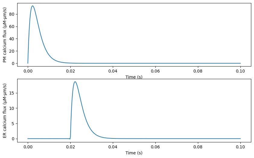
We can plot the time-dependent stimulus from r1 and r2 using lambdify.
from sympy.utilities.lambdify import lambdify
pulsePM_func = lambdify(t, pulsePM, 'numpy')  # returns a numpy-ready function
pulseER_func = lambdify(t, pulseER, 'numpy')
tArray = np.linspace(0, 0.1, 500)
fig, ax = plt.subplots(2, 1)
fig.set_size_inches(10, 6)
ax[0].plot(tArray, pulsePM_func(tArray))
ax[0].set(xlabel='Time (s)',
          ylabel='PM calcium flux (μM-μm/s)')
ax[1].plot(tArray, pulseER_func(tArray))
ax[1].set(xlabel='Time (s)',
          ylabel='ER calcium flux (μM-μm/s)')
[Text(0.5, 0, 'Time (s)'), Text(0, 0.5, 'ER calcium flux (μM-μm/s)')]
Create and load in mesh#
Here, we consider an “ellipsoid-in-an-ellipsoid” geometry. The inner ellipsoid represents the ER and the volume between the ER boundary and the boundary of the outer ellipsoid represents the cytosol.
curRadius = 0.25  # dendritic spine radius
domain, facet_markers, cell_markers = mesh_tools.create_ellipsoids((1.25*curRadius, 0.8*curRadius, curRadius),
                                                                   (1.25*curRadius/2, 0.8 *
                                                                    curRadius/2, curRadius/2),
                                                                   hEdge=0.01)
# Write mesh and meshfunctions to file
mesh_folder = pathlib.Path("mesh")
mesh_folder.mkdir(exist_ok=True)
mesh_path = mesh_folder / "DemoEllipsoid.h5"
mesh_tools.write_mesh(
    domain, facet_markers, cell_markers, filename=mesh_path
)
parent_mesh = mesh.ParentMesh(
    mesh_filename=str(mesh_path),
    mesh_filetype="hdf5",
    name="parent_mesh",
)
visualization.plot_dolfin_mesh(domain, cell_markers, facet_markers)
2026-03-05 08:18:12,968 smart.mesh - INFO - HDF5 mesh, "parent_mesh", successfully loaded from file: mesh/DemoEllipsoid.h5! (mesh.py:245)
2026-03-05 08:18:12,968 smart.mesh - INFO - 0 subdomains successfully loaded from file: mesh/DemoEllipsoid.h5! (mesh.py:258)
/usr/lib/python3/dist-packages/smart/visualization.py:283: PyVistaDeprecationWarning: This function is deprecated and will be removed in future version of PyVista. Use vtk with osmesa instead.
  pyvista.start_xvfb()
ROOT -2026-03-05 08:18:18,032 trame_server.utils.namespace - INFO - Translator(prefix=None) (namespace.py:65)
ROOT -2026-03-05 08:18:18,077 wslink.backends.aiohttp - INFO - awaiting runner setup (__init__.py:147)
ROOT -2026-03-05 08:18:18,078 wslink.backends.aiohttp - INFO - awaiting site startup (__init__.py:154)
ROOT -2026-03-05 08:18:18,079 wslink.backends.aiohttp - INFO - Print WSLINK_READY_MSG (__init__.py:160)
ROOT -2026-03-05 08:18:18,080 wslink.backends.aiohttp - INFO - Schedule auto shutdown with timeout 0 (__init__.py:166)
ROOT -2026-03-05 08:18:18,080 wslink.backends.aiohttp - INFO - awaiting running future (__init__.py:169)
Initialize model and solver.
config_cur = config.Config()
config_cur.flags.update({"allow_unused_components": True})
model_cur = model.Model(pc, sc, cc, rc, config_cur, parent_mesh)
config_cur.solver.update(
    {
        "final_t": 0.1,
        "initial_dt": 0.001,
        "time_precision": 6,
    }
)
model_cur.initialize()
2026-03-05 08:18:25,362 smart.solvers - INFO - Jpetsc_nest assembled, size = (19735, 19735) (solvers.py:201)
2026-03-05 08:18:25,363 smart.solvers - INFO - Initializing block residual vector (solvers.py:209)
 2026-03-05 08:18:25,557 smart.model_assembly - INFO -
╒═════════╤════════════════════════════════════════════════════════════════════════════════════════════════════════════════════════════╤═══════════════╕
│         │ Value/Equation                                                                                                             │ Description   │
╞═════════╪════════════════════════════════════════════════════════════════════════════════════════════════════════════════════════════╪═══════════════╡
│ j1pulse │ -1140.0*exp(-500.0*t) + 1140.0*exp(-400.0*t) µm·µM/s                                                                       │               │
├─────────┼────────────────────────────────────────────────────────────────────────────────────────────────────────────────────────────┼───────────────┤
│ j2pulse │ 228.0*(-22026.4657948067*exp(-500.0*t) + 2980.95798704173*exp(-400.0*t))/(1 + 5.22146968976414e+173*exp(-20000*t)) µm·µM/s │               │
├─────────┼────────────────────────────────────────────────────────────────────────────────────────────────────────────────────────────┼───────────────┤
│ tau     │ 5.00×10⁻² s                                                                                                                │               │
╘═════════╧════════════════════════════════════════════════════════════════════════════════════════════════════════════════════════════╧═══════════════╛
 (model_assembly.py:371)
 2026-03-05 08:18:25,560 smart.model_assembly - INFO -
╒════╤═══════════════╤════════════════╤═════════════════════╕
│    │ Compartment   │ D              │ Initial condition   │
╞════╪═══════════════╪════════════════╪═════════════════════╡
│ Ca │ Cyto          │ 1.00×10¹ µm²/s │ 5.00×10⁻² µM        │
╘════╧═══════════════╧════════════════╧═════════════════════╛
 (model_assembly.py:371)
 2026-03-05 08:18:25,572 smart.model_assembly - INFO -
╒══════╤══════════════════╤═══════════╤════════════╤═════════╤════════════════╤═══════════════╕
│      │   Dimensionality │   Species │   Vertices │   Cells │   Marker value │ Size          │
╞══════╪══════════════════╪═══════════╪════════════╪═════════╪════════════════╪═══════════════╡
│ Cyto │                3 │         1 │      19735 │   86686 │              1 │ 5.74×10⁻² µm³ │
├──────┼──────────────────┼───────────┼────────────┼─────────┼────────────────┼───────────────┤
│ PM   │                2 │         0 │      10705 │   21406 │             10 │ 8.06×10⁻¹ µm² │
├──────┼──────────────────┼───────────┼────────────┼─────────┼────────────────┼───────────────┤
│ ERm  │                2 │         0 │        289 │     574 │             12 │ 1.99×10⁻¹ µm² │
╘══════╧══════════════════╧═══════════╧════════════╧═════════╧════════════════╧═══════════════╛
 (model_assembly.py:371)
 2026-03-05 08:18:25,587 smart.model_assembly - INFO -
╒════╤═════════════╤════════════╤════════════╤════════════════╕
│    │ Reactants   │ Products   │ Equation   │ Type           │
╞════╪═════════════╪════════════╪════════════╪════════════════╡
│ r1 │ []          │ ['Ca']     │ j1pulse    │ volume_surface │
├────┼─────────────┼────────────┼────────────┼────────────────┤
│ r2 │ []          │ ['Ca']     │ j2pulse    │ volume_surface │
├────┼─────────────┼────────────┼────────────┼────────────────┤
│ r3 │ ['Ca']      │ []         │ Ca/tau     │ volume         │
╘════╧═════════════╧════════════╧════════════╧════════════════╛
 (model_assembly.py:371)
╒════╤═════════════╤══════╤══════════════════╤═════════════╤══════════════╤════════════════╕
│    │ name        │   id │   dimensionality │   num_cells │   num_facets │   num_vertices │
╞════╪═════════════╪══════╪══════════════════╪═════════════╪══════════════╪════════════════╡
│  0 │ parent_mesh │   16 │                3 │       88107 │       186917 │          19843 │
├────┼─────────────┼──────┼──────────────────┼─────────────┼──────────────┼────────────────┤
│  1 │ Cyto        │   40 │                3 │       86686 │       184362 │          19735 │
├────┼─────────────┼──────┼──────────────────┼─────────────┼──────────────┼────────────────┤
│  2 │ PM          │   47 │                2 │       21406 │        32109 │          10705 │
├────┼─────────────┼──────┼──────────────────┼─────────────┼──────────────┼────────────────┤
│  3 │ ERm         │   54 │                2 │         574 │          861 │            289 │
╘════╧═════════════╧══════╧══════════════════╧═════════════╧══════════════╧════════════════╛
Initialize XDMF files for saving results, save model information to .pkl file, then solve the system until model_cur.t > model_cur.final_t
# Write initial condition(s) to file
results = dict()
result_folder = pathlib.Path(f"results")
result_folder.mkdir(exist_ok=True)
for species_name, species in model_cur.sc.items:
    results[species_name] = d.XDMFFile(
        model_cur.mpi_comm_world, str(result_folder / f"{species_name}.xdmf")
    )
    results[species_name].parameters["flush_output"] = True
    results[species_name].write(model_cur.sc[species_name].u["u"], model_cur.t)
model_cur.to_pickle("model_cur.pkl")

# Set loglevel to warning in order not to pollute notebook output
logger.setLevel(logging.WARNING)

concVec = np.array([.05])
cytoMesh = model_cur.cc['Cyto'].dolfin_mesh
integrateDomain = d.MeshFunction("size_t", cytoMesh, 3, 0)
RTarget = (curRadius + curRadius/2) / 2
for c in d.cells(cytoMesh):
    RCur = np.sqrt(c.midpoint().x()**2 + c.midpoint().y()**2 + c.midpoint().z()**2)
    integrateDomain[c] = 1 if (RCur > RTarget-.1*curRadius and RCur <
                                RTarget + .1*curRadius) else 0
dx = d.Measure("dx", domain=cytoMesh, subdomain_data=integrateDomain)
volume = d.assemble_mixed(1.0*dx(1))
# Solve
displayed = False
while True:
    # Solve the system
    model_cur.monolithic_solve()
    # Save results for post processing
    for species_name, species in model_cur.sc.items:
        results[species_name].write(model_cur.sc[species_name].u["u"], model_cur.t)
    # save mean value at r = (curRadius + curRadius/2)/2 (for comparison to Cugno graph below)
    int_val = d.assemble_mixed(model_cur.sc['Ca'].u['u']*dx(1))
    curConc = np.array([int_val / volume])
    concVec = np.concatenate((concVec, curConc))
    np.savetxt(result_folder / f"tvec.txt", np.array(model_cur.tvec).astype(np.float32))
    if model_cur.t > .025 and not displayed:  # display first time after .025 s
        visualization.plot(model_cur.sc['Ca'].u['u'])
        displayed = True
    # End if we've passed the final time
    if model_cur.t >= model_cur.final_t:
        break
/usr/lib/python3/dist-packages/smart/visualization.py:167: PyVistaDeprecationWarning: This function is deprecated and will be removed in future version of PyVista. Use vtk with osmesa instead.
  pyvista.start_xvfb()
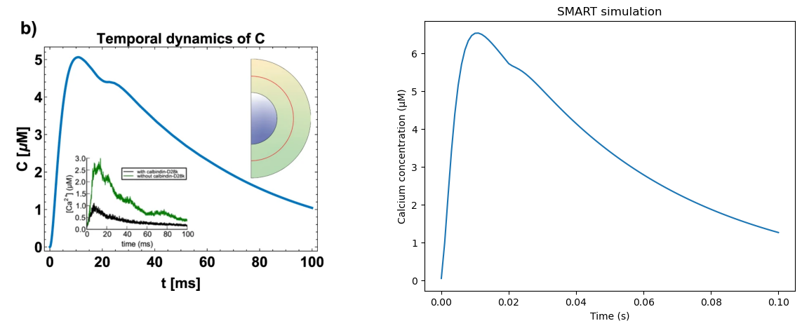
Plot results side-by-side with figure from original paper. This graph from the paper uses a spherical cell geometry, whereas we use an ellipsoidal case here, so we expect only qualitatively similar dynamics.
rcParams['figure.figsize'] = 15, 5
# read image from Fig 3b of paper
img_A = mpimg.imread('Cugno_et_al_2019_Fig3b.png')
fig, ax = plt.subplots(1, 2)
ax[0].imshow(img_A)
ax[0].axis('off')
ax[1].plot(model_cur.tvec, concVec)
plt.xlabel("Time (s)")
plt.ylabel("Calcium concentration (μM)")
plt.title("SMART simulation")
Text(0.5, 1.0, 'SMART simulation')
Compare area under the curve (AUC) with value from previous simulations (regression test).
tvec = np.zeros(len(model_cur.tvec))
for i in range(len(model_cur.tvec)):
    tvec[i] = float(model_cur.tvec[i])
auc_cur = np.trapz(concVec, tvec)
auc_compare = 0.35133404882191754
percent_error = 100*np.abs(auc_cur - auc_compare)/auc_compare
assert percent_error < .012,\
    f"Failed regression test: Example 4 results deviate {percent_error:.3f}% from the previous numerical solution"