Example 2: Simple 2D cell signaling model

We model a reaction between the cell interior and cell membrane in a 2D geometry:

• Cyto - 2D cell “volume”

• PM - 1D cell boundary (represents plasma membrane)

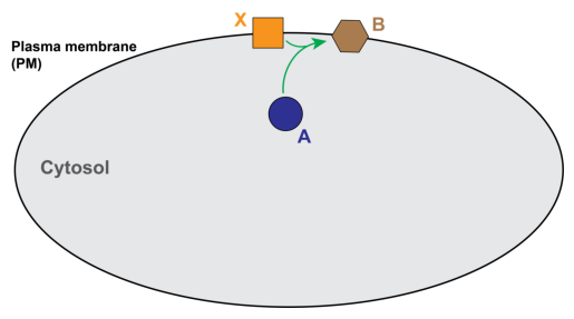
Model from Rangamani et al, 2013, Cell. A cytosolic species, “A”, reacts with a species on the PM, “B”, to form a new species on the PM, “X”. The resulting PDE and boundary condition for species A are as follows:

\[\begin{split} \frac{\partial{C_A}}{\partial{t}} = D_A \nabla ^2 C_A \quad \text{in} \; \Omega_{Cyto}\\ \text{B.C. for A:} \quad D_A (\textbf{n} \cdot \nabla C_A) = -k_{on} C_A N_X + k_{off} N_B \quad \text{on} \; \Gamma_{PM} \end{split}\]

Similarly, the PDEs for X and B are given by: $\( \frac{\partial{N_X}}{\partial{t}} = D_X \nabla ^2 N_X - k_{on} C_A N_X + k_{off} N_B \quad \text{on} \; \Gamma_{PM}\\ \frac{\partial{N_B}}{\partial{t}} = D_B \nabla ^2 N_B + k_{on} C_A N_X - k_{off} N_B \quad \text{on} \; \Gamma_{PM} \)$

from matplotlib import pyplot as plt
import matplotlib.image as mpimg
img_A = mpimg.imread('axb-diagram.png')
plt.imshow(img_A)
plt.axis('off')

(-0.5, 5830.5, 3140.5, -0.5)

Imports and logger initialization:

import dolfin as d
import sympy as sym
import numpy as np
import pathlib
import logging
import gmsh  # must be imported before pyvista if dolfin is imported first

from smart import config, common, mesh, model, mesh_tools, visualization
from smart.units import unit
from smart.model_assembly import (
    Compartment,
    Parameter,
    Reaction,
    Species,
    SpeciesContainer,
    ParameterContainer,
    CompartmentContainer,
    ReactionContainer,
)
from matplotlib import pyplot as plt
import matplotlib.image as mpimg

logger = logging.getLogger("smart")
logger.setLevel(logging.INFO)

/usr/lib/python3/dist-packages/scipy/__init__.py:146: UserWarning: A NumPy version >=1.17.3 and <1.25.0 is required for this version of SciPy (detected version 1.26.4
  warnings.warn(f"A NumPy version >={np_minversion} and <{np_maxversion}"

First, we define the various units for use in the model.

um = unit.um
molecule = unit.molecule
sec = unit.sec
dimensionless = unit.dimensionless
D_unit = um**2 / sec
surf_unit = molecule / um**2
flux_unit = molecule / (um * sec)
edge_unit = molecule / um

Next we generate the model by assembling the compartment, species, parameter, and reaction containers (see Example 1 or API documentation for more details).

# =============================================================================================
# Compartments
# =============================================================================================
# name, topological dimensionality, length scale units, marker value
Cyto = Compartment("Cyto", 2, um, 1)
PM = Compartment("PM", 1, um, 3)
cc = CompartmentContainer()
cc.add([Cyto, PM])

# =============================================================================================
# Species
# =============================================================================================
# name, initial concentration, concentration units, diffusion, diffusion units, compartment
A = Species("A", 1.0, surf_unit, 100.0, D_unit, "Cyto")
X = Species("X", 1.0, edge_unit, 1.0, D_unit, "PM")
B = Species("B", 0.0, edge_unit, 1.0, D_unit, "PM")
sc = SpeciesContainer()
sc.add([A, X, B])

# =============================================================================================
# Parameters and Reactions
# =============================================================================================

# Reaction of A and X to make B (Cyto-PM reaction)
kon = Parameter("kon", 1.0, 1/(surf_unit*sec))
koff = Parameter("koff", 1.0, 1/sec)
r1 = Reaction("r1", ["A", "X"], ["B"],
              param_map={"on": "kon", "off": "koff"},
              species_map={"A": "A", "X": "X", "B": "B"})

pc = ParameterContainer()
pc.add([kon, koff])
rc = ReactionContainer()
rc.add([r1])

Now we create a circular mesh (mesh built using gmsh in smart.mesh_tools), along with marker functions mf2 and mf1.

# Create mesh
h_ellipse = 0.1
xrad = 1.0
yrad = 1.0
surf_tag = 1
edge_tag = 3
ellipse_mesh, mf1, mf2 = mesh_tools.create_ellipses(xrad, yrad, hEdge=h_ellipse,
                                                    outer_tag=surf_tag, outer_marker=edge_tag)
visualization.plot_dolfin_mesh(ellipse_mesh, mf2, view_xy=True)

Info    : Meshing 1D...
Info    : Meshing curve 1 (Ellipse)
Info    : Done meshing 1D (Wall 0.00948801s, CPU 0.00291s)
Info    : Meshing 2D...
Info    : Meshing surface 1 (Plane, Delaunay)
Info    : Done meshing 2D (Wall 0.0365626s, CPU 0.036592s)
Info    : 455 nodes 909 elements
Info    : Writing 'tmp_ellipse_[1.0, 1.0]_[0.0, 0.0]_0/ellipses.msh'...
Info    : Done writing 'tmp_ellipse_[1.0, 1.0]_[0.0, 0.0]_0/ellipses.msh'

Write mesh and meshfunctions to file, then create mesh.ParentMesh object.

mesh_folder = pathlib.Path("ellipse_mesh_AR1")
mesh_folder.mkdir(exist_ok=True)
mesh_file = mesh_folder / "ellipse_mesh.h5"
mesh_tools.write_mesh(ellipse_mesh, mf1, mf2, mesh_file)

parent_mesh = mesh.ParentMesh(
    mesh_filename=str(mesh_file),
    mesh_filetype="hdf5",
    name="parent_mesh",
)

 2024-05-07 12:05:31,456 smart.mesh - INFO - HDF5 mesh, "parent_mesh", successfully loaded from file: ellipse_mesh_AR1/ellipse_mesh.h5! (mesh.py:245) 

 2024-05-07 12:05:31,457 smart.mesh - INFO - 0 subdomains successfully loaded from file: ellipse_mesh_AR1/ellipse_mesh.h5! (mesh.py:258) 

Initialize model and solvers.

config_cur = config.Config()
config_cur.solver.update(
    {
        "final_t": 10.0,
        "initial_dt": 0.05,
        "time_precision": 6,
    }
)

model_cur = model.Model(pc, sc, cc, rc, config_cur, parent_mesh)
model_cur.initialize()

 2024-05-07 12:05:38,180 smart.model - WARNING - Warning! Initial L2-norm of compartment PM is 1.119037357695821 (possibly too large). (model.py:1179) 

 2024-05-07 12:05:38,184 smart.solvers - INFO - Jpetsc_nest assembled, size = (581, 581) (solvers.py:199) 

 2024-05-07 12:05:38,185 smart.solvers - INFO - Initializing block residual vector (solvers.py:207) 

 2024-05-07 12:05:38,193 smart.model_assembly - INFO - 
╒══════╤═════════════════════════╤═════════════════════╤════════════╤═════════╤═════════╕
│      │ quantity                │ is_time_dependent   │ sym_expr   │ notes   │ group   │
╞══════╪═════════════════════════╪═════════════════════╪════════════╪═════════╪═════════╡
│ kon  │ 1.00×10⁰ µm²/molecule/s │ False               │            │         │         │
├──────┼─────────────────────────┼─────────────────────┼────────────┼─────────┼─────────┤
│ koff │ 1.00×10⁰ 1/s            │ False               │            │         │         │
╘══════╧═════════════════════════╧═════════════════════╧════════════╧═════════╧═════════╛
 (model_assembly.py:337) 

 2024-05-07 12:05:38,198 smart.model_assembly - INFO - 
╒════╤════════════════════╤════════════════╤═════════════════════╤═══════════════════════╕
│    │ compartment_name   │ Diffusion      │   initial_condition │ concentration_units   │
╞════╪════════════════════╪════════════════╪═════════════════════╪═══════════════════════╡
│ A  │ Cyto               │ 1.00×10² µm²/s │                   1 │ 1.00×10⁰ molecule/µm² │
├────┼────────────────────┼────────────────┼─────────────────────┼───────────────────────┤
│ X  │ PM                 │ 1.00×10⁰ µm²/s │                   1 │ 1.00×10⁰ molecule/µm  │
├────┼────────────────────┼────────────────┼─────────────────────┼───────────────────────┤
│ B  │ PM                 │ 1.00×10⁰ µm²/s │                   0 │ 1.00×10⁰ molecule/µm  │
╘════╧════════════════════╧════════════════╧═════════════════════╧═══════════════════════╛
 (model_assembly.py:337) 

 2024-05-07 12:05:38,568 smart.model_assembly - INFO - 
╒══════╤══════════════════╤═══════════════╤════════════════╤════════════╤═════════════╤═══════════════╤══════════════╕
│      │   dimensionality │   num_species │   num_vertices │   num_dofs │   num_cells │   cell_marker │ nvolume      │
╞══════╪══════════════════╪═══════════════╪════════════════╪════════════╪═════════════╪═══════════════╪══════════════╡
│ Cyto │                2 │             1 │            455 │        455 │         845 │             1 │ 3.14×10⁰ µm² │
├──────┼──────────────────┼───────────────┼────────────────┼────────────┼─────────────┼───────────────┼──────────────┤
│ PM   │                1 │             2 │             63 │        126 │          63 │             3 │ 6.28×10⁰ µm  │
╘══════╧══════════════════╧═══════════════╧════════════════╧════════════╧═════════════╧═══════════════╧══════════════╛
 (model_assembly.py:337) 

 2024-05-07 12:05:38,573 smart.model_assembly - INFO - 
╒════╤════════════╤═══════╤═════════════╤═════════════╕
│    │ lhs        │ rhs   │ eqn_f_str   │ eqn_r_str   │
╞════╪════════════╪═══════╪═════════════╪═════════════╡
│ r1 │ ['A', 'X'] │ ['B'] │ kon*A*X     │ koff*B      │
╘════╧════════════╧═══════╧═════════════╧═════════════╛
 (model_assembly.py:337) 

╒════╤═════════════╤══════╤══════════════════╤═════════════╤══════════════╤════════════════╕
│    │ name        │   id │   dimensionality │   num_cells │   num_facets │   num_vertices │
╞════╪═════════════╪══════╪══════════════════╪═════════════╪══════════════╪════════════════╡
│  0 │ parent_mesh │   18 │                2 │         845 │         1299 │            455 │
├────┼─────────────┼──────┼──────────────────┼─────────────┼──────────────┼────────────────┤
│  1 │ Cyto        │   32 │                2 │         845 │         1299 │            455 │
├────┼─────────────┼──────┼──────────────────┼─────────────┼──────────────┼────────────────┤
│  2 │ PM          │   39 │                1 │          63 │           63 │             63 │
╘════╧═════════════╧══════╧══════════════════╧═════════════╧══════════════╧════════════════╛

Save model information to .pkl file and write initial conditions to file.

model_cur.to_pickle('model_cur.pkl')
results = dict()
result_folder = pathlib.Path("resultsEllipse_AR1_loaded")
result_folder.mkdir(exist_ok=True)
for species_name, species in model_cur.sc.items:
    results[species_name] = d.XDMFFile(
        model_cur.mpi_comm_world, str(result_folder / f"{species_name}.xdmf")
    )
    results[species_name].parameters["flush_output"] = True
    results[species_name].write(model_cur.sc[species_name].u["u"], model_cur.t)

Solve the system until model_cur.t > model_cur.final_t.

tvec = [0]
avg_A = [A.initial_condition]
# Set loglevel to warning in order not to pollute notebook output
logger.setLevel(logging.WARNING)

while True:
    # Solve the system
    model_cur.monolithic_solve()
    # Save results for post processing
    for species_name, species in model_cur.sc.items:
        results[species_name].write(model_cur.sc[species_name].u["u"], model_cur.t)
    dx = d.Measure("dx", domain=model_cur.cc['Cyto'].dolfin_mesh)
    int_val = d.assemble_mixed(model_cur.sc['A'].u['u']*dx)
    volume = d.assemble_mixed(1.0*dx)
    avg_A.append(int_val / volume)
    tvec.append(model_cur.t)
    # End if we've passed the final time
    if model_cur.t >= model_cur.final_t:
        break

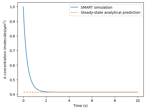
Now we plot the concentration of A in the cell over time and compare this to analytical predictions for a high value of the diffusion coefficient. As \(D_A \rightarrow \infty\), the steady state concentration of A will be given by the positive root of the following polynomial:

\[ -k_{on} c_A ^2 - \left( k_{on} c_{X} (t=0) \frac{SA_{PM}}{vol_{cyto}} + k_{off} - k_{on} c_A (t=0) \right) c_A + k_{off} c_A(t=0) \]

Note that in this 2D case, \(SA_{PM}\) is the perimeter of the ellipse and \(vol_{cyto}\) is the area of the ellipse. These can be thought of as a surface area and volume if we extrude the 2D shape by some characteristic thickness.

plt.plot(tvec, avg_A, label='SMART simulation')
plt.xlabel('Time (s)')
plt.ylabel('A concentration $\mathrm{(molecules/μm^2)}$')
SA_vol = 4/(xrad + yrad)
root_vals = np.roots([-kon.value,
                      -kon.value*X.initial_condition*SA_vol - koff.value + kon.value*A.initial_condition,
                      koff.value*A.initial_condition])
ss_pred = root_vals[root_vals > 0]
plt.plot(tvec, np.ones(len(avg_A))*ss_pred, '--', label='Steady-state analytical prediction')
plt.legend()
percent_error_analytical = 100*np.abs(ss_pred-avg_A[-1])/ss_pred
assert percent_error_analytical < 0.1,\
    f"Failed test: Example 2 results deviate {percent_error_analytical:.3f}% from the analytical prediction"

Plot A concentration in the cell at the final time point.

visualization.plot(model_cur.sc["A"].u["u"], view_xy=True)
# also save to file for comparison visualization in the end
meshimg_folder = pathlib.Path("mesh_images")
meshimg_folder = meshimg_folder.resolve()
meshimg_folder.mkdir(exist_ok=True)
meshimg_file = meshimg_folder / "ellipse_mesh_AR1.png"

# Put all images in a dictionary for easy recovery later
images = {}
images[1] = visualization.plot(model_cur.sc["A"].u["u"], view_xy=True, filename=meshimg_file)

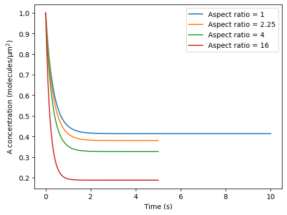
Now iterate over three different cell aspect ratios and compare dynamics between cases.

# initialize plot to compare dynamics
plt.plot(tvec, avg_A, label='Aspect ratio = 1')
plt.xlabel('Time (s)')
plt.ylabel('A concentration $\mathrm{(molecules/μm^2)}$')
# iterate over additional aspect ratios, enforcing the same ellipsoid area in all cases
aspect_ratios = [1, 1.5**2, 4, 16]
ss_calc = [avg_A[-1]]
for i in range(1, len(aspect_ratios)):
    # Create mesh
    xrad = 1.0*np.sqrt(aspect_ratios[i])
    yrad = 1.0/np.sqrt(aspect_ratios[i])
    ellipse_mesh, mf1, mf2 = mesh_tools.create_ellipses(xrad, yrad, hEdge=h_ellipse,
                                                        outer_tag=surf_tag, outer_marker=edge_tag)
    mesh_folder = pathlib.Path(f"ellipse_mesh_AR{aspect_ratios[i]}")
    mesh_folder.mkdir(exist_ok=True)
    mesh_tools.write_mesh(ellipse_mesh, mf1, mf2, mesh_file)
    parent_mesh = mesh.ParentMesh(
        mesh_filename=str(mesh_file),
        mesh_filetype="hdf5",
        name="parent_mesh",
    )
    config_cur = config.Config()
    config_cur.solver.update(
        {
            "final_t": 5.0,
            "initial_dt": 0.05,
            "time_precision": 6,
        }
    )
    model_cur = model.Model(pc, sc, cc, rc, config_cur, parent_mesh)
    model_cur.initialize()
    results = dict()
    result_folder = pathlib.Path(f"resultsEllipse_AR{aspect_ratios[i]}")
    result_folder.mkdir(exist_ok=True)
    for species_name, species in model_cur.sc.items:
        results[species_name] = d.XDMFFile(
            model_cur.mpi_comm_world, str(result_folder / f"{species_name}.xdmf")
        )
        results[species_name].parameters["flush_output"] = True
        results[species_name].write(model_cur.sc[species_name].u["u"], model_cur.t)
    avg_A = [A.initial_condition]
    dx = d.Measure("dx", domain=model_cur.cc['Cyto'].dolfin_mesh)
    volume = d.assemble_mixed(1.0*dx)
    while True:
        # Solve the system
        model_cur.monolithic_solve()
        # Save results for post processing
        for species_name, species in model_cur.sc.items:
            results[species_name].write(model_cur.sc[species_name].u["u"], model_cur.t)
        int_val = d.assemble_mixed(model_cur.sc['A'].u['u']*dx)
        avg_A.append(int_val / volume)
        # End if we've passed the final time
        if model_cur.t >= model_cur.final_t:
            break
    plt.plot(model_cur.tvec, avg_A, label=f"Aspect ratio = {aspect_ratios[i]}")
    ss_calc.append(avg_A[-1])
    meshimg_file = meshimg_folder / f"ellipse_mesh_AR{aspect_ratios[i]}.png"
    images[aspect_ratios[i]] = visualization.plot(model_cur.sc["A"].u["u"], view_xy=True, filename=meshimg_file)
plt.legend()

Info    : Meshing 1D...
Info    : Meshing curve 1 (Ellipse)

Info    : Done meshing 1D (Wall 0.486481s, CPU 0.480736s)
Info    : Meshing 2D...
Info    : Meshing surface 1 (Plane, Delaunay)
Info    : Done meshing 2D (Wall 0.0365145s, CPU 0.036871s)
Info    : 446 nodes 891 elements
Info    : Writing 'tmp_ellipse_[1.5, 0.6666666666666666]_[0.0, 0.0]_0/ellipses.msh'...
Info    : Done writing 'tmp_ellipse_[1.5, 0.6666666666666666]_[0.0, 0.0]_0/ellipses.msh'

 2024-05-07 12:05:49,889 smart.model - WARNING - Warning! Initial L2-norm of compartment PM is 1.184345213443547 (possibly too large). (model.py:1179) 

╒════╤═════════════╤═══════╤══════════════════╤═════════════╤══════════════╤════════════════╕
│    │ name        │    id │   dimensionality │   num_cells │   num_facets │   num_vertices │
╞════╪═════════════╪═══════╪══════════════════╪═════════════╪══════════════╪════════════════╡
│  0 │ parent_mesh │ 12122 │                2 │         819 │         1264 │            446 │
├────┼─────────────┼───────┼──────────────────┼─────────────┼──────────────┼────────────────┤
│  1 │ Cyto        │ 12136 │                2 │         819 │         1264 │            446 │
├────┼─────────────┼───────┼──────────────────┼─────────────┼──────────────┼────────────────┤
│  2 │ PM          │ 12143 │                1 │          71 │           71 │             71 │
╘════╧═════════════╧═══════╧══════════════════╧═════════════╧══════════════╧════════════════╛

Info    : Meshing 1D...
Info    : Meshing curve 1 (Ellipse)

 2024-05-07 12:05:56,144 smart.model - WARNING - Warning! Initial L2-norm of compartment PM is 1.3068209611994575 (possibly too large). (model.py:1179) 

Info    : Done meshing 1D (Wall 0.591992s, CPU 0.570527s)
Info    : Meshing 2D...
Info    : Meshing surface 1 (Plane, Delaunay)
Info    : Done meshing 2D (Wall 0.0401177s, CPU 0.040514s)
Info    : 457 nodes 913 elements
Info    : Writing 'tmp_ellipse_[2.0, 0.5]_[0.0, 0.0]_0/ellipses.msh'...
Info    : Done writing 'tmp_ellipse_[2.0, 0.5]_[0.0, 0.0]_0/ellipses.msh'

╒════╤═════════════╤═══════╤══════════════════╤═════════════╤══════════════╤════════════════╕
│    │ name        │    id │   dimensionality │   num_cells │   num_facets │   num_vertices │
╞════╪═════════════╪═══════╪══════════════════╪═════════════╪══════════════╪════════════════╡
│  0 │ parent_mesh │ 19179 │                2 │         826 │         1282 │            457 │
├────┼─────────────┼───────┼──────────────────┼─────────────┼──────────────┼────────────────┤
│  1 │ Cyto        │ 19193 │                2 │         826 │         1282 │            457 │
├────┼─────────────┼───────┼──────────────────┼─────────────┼──────────────┼────────────────┤
│  2 │ PM          │ 19200 │                1 │          86 │           86 │             86 │
╘════╧═════════════╧═══════╧══════════════════╧═════════════╧══════════════╧════════════════╛

Info    : Meshing 1D...
Info    : Meshing curve 1 (Ellipse)

 2024-05-07 12:06:02,700 smart.model - WARNING - Warning! Initial L2-norm of compartment Cyto is 1.264749048952121 (possibly too large). (model.py:1179) 

 2024-05-07 12:06:02,702 smart.model - WARNING - Warning! Initial L2-norm of compartment PM is 1.7886252580265631 (possibly too large). (model.py:1179) 

Info    : Done meshing 1D (Wall 0.745804s, CPU 0.740057s)
Info    : Meshing 2D...
Info    : Meshing surface 1 (Plane, Delaunay)
Info    : Done meshing 2D (Wall 0.0531543s, CPU 0.053458s)
Info    : 471 nodes 941 elements
Info    : Writing 'tmp_ellipse_[4.0, 0.25]_[0.0, 0.0]_0/ellipses.msh'...
Info    : Done writing 'tmp_ellipse_[4.0, 0.25]_[0.0, 0.0]_0/ellipses.msh'

╒════╤═════════════╤═══════╤══════════════════╤═════════════╤══════════════╤════════════════╕
│    │ name        │    id │   dimensionality │   num_cells │   num_facets │   num_vertices │
╞════╪═════════════╪═══════╪══════════════════╪═════════════╪══════════════╪════════════════╡
│  0 │ parent_mesh │ 26236 │                2 │         778 │         1248 │            471 │
├────┼─────────────┼───────┼──────────────────┼─────────────┼──────────────┼────────────────┤
│  1 │ Cyto        │ 26250 │                2 │         778 │         1248 │            471 │
├────┼─────────────┼───────┼──────────────────┼─────────────┼──────────────┼────────────────┤
│  2 │ PM          │ 26257 │                1 │         162 │          162 │            162 │
╘════╧═════════════╧═══════╧══════════════════╧═════════════╧══════════════╧════════════════╛

<matplotlib.legend.Legend at 0x7f66a0bfa590>

Compare steady-state values with those from past runs using SMART (regression test):

ss_stored = [0.41384929369203755, 0.38021621231324093, 0.32689497127690803, 0.18803994874948224]
percent_error = max(np.abs(np.array(ss_stored) - np.array(ss_calc))/np.array(ss_stored))*100
assert percent_error < .01,\
    f"Failed regression test: Example 2 results deviate {percent_error:.3f}% from the previous numerical solution"

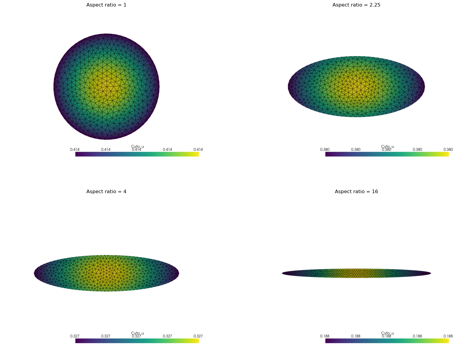
Now, display the final states from all simulations for direct comparison.

fig, ax = plt.subplots(2, 2, figsize=(20, 15))
for axi, (aspect_ratio, image) in zip(ax.flatten(), images.items()):
    axi.imshow(image)
    axi.axis('off')
    axi.set_title(f"Aspect ratio = {aspect_ratio}")