Example 3: Protein phosphorylation and diffusion in 3D cell geometry#
Here, we implement the model of protein phosphorylation at the cell membrane and diffusion in the cytosol from Meyers, Craig, and Odde 2006, Current Biology.
This model geometry consists of 2 domains - one surface and one volume:
plasma membrane (PM) - cell surface
cytosol - intracellular volume
In this case, we only model the case of a spherical cell, where the cytosol corresponds to the interior of the sphere and the PM corresponds to the surface of the sphere.
This model includes a single species, A, which is phosphorylated at the cell membrane. The unphosphorylated form of A (\(A_{dephos}\)) can be computed from mass conservation; everywhere \(c_{A_{phos}} + c_{A_{dephos}} = c_{Tot}\), which is a constant in both time and space if the phosphorylated vs. unphosphorylated forms have the same diffusion coefficient.
There are two reactions - one in the PM and other in the cytosol. At the membrane, \(A_{dephos}\) is phosphorylated by a first-order reaction with rate \(k_{kin}\), and in the cytosolic volume, \(A_{phos}\) is dephosphorylated by a first order reaction with rate \(k_p\). The resulting equations are:
where we note that \(c_{A_{dephos}} = c_{Tot} - c_{A_{phos}}\) in the boundary condition due to mass conservation.
In this file, we test this model over multiple cell sizes and compare the results to analytical predictions. Please note that because we are testing several different geometries, this file may take an hour or more to complete execution.
import dolfin as d
import numpy as np
import pathlib
import logging

from smart import config, mesh, model, mesh_tools
from smart.units import unit
import sympy as sym
import gmsh  # must be imported before pyvista if dolfin is imported first

from smart import config, common, mesh, model, mesh_tools, visualization
from smart.model_assembly import (
    Compartment,
    Parameter,
    Reaction,
    Species,
    SpeciesContainer,
    ParameterContainer,
    CompartmentContainer,
    ReactionContainer,
)

from matplotlib import pyplot as plt
import matplotlib.image as mpimg
from matplotlib import rcParams
/usr/lib/python3/dist-packages/scipy/__init__.py:146: UserWarning: A NumPy version >=1.17.3 and <1.25.0 is required for this version of SciPy (detected version 1.26.4
  warnings.warn(f"A NumPy version >={np_minversion} and <{np_maxversion}"
We will set the logging level to INFO. This will display some output during the simulation. If you want to get even more output you could set the logging level to DEBUG.
logger = logging.getLogger("smart")
logger.setLevel(logging.INFO)
Futhermore, you could also save the logs to a file by attaching a file handler to the logger as follows.
file_handler = logging.FileHandler("filename.log")
file_handler.setFormatter(logging.Formatter(smart.config.base_format))
logger.addHandler(file_handler)
Now, we define various units used in this problem.
uM = unit.uM
um = unit.um
molecule = unit.molecule
sec = unit.sec
dimensionless = unit.dimensionless
D_unit = um**2 / sec
flux_unit = molecule / (um**2 * sec)
vol_unit = uM
Generate model#
Next we generate the model, which consists of four containers - compartments, species, reactions, and parameters.
Compartments#
As described above, the two compartments are the cytosol (“Cyto”) and the plasma membrane (“PM”). These are initialized by calling:
compartment_var = Compartment(name, dimensionality, compartment_units, cell_marker)
where
name: string naming the compartment
dimensionality: topological dimensionality (i.e. 3 for Cyto, 2 for PM)
compartment_units: length units for the compartment (um for both here)
cell_marker: integer marker value identifying each compartment in the parent mesh
Cyto = Compartment("Cyto", 3, um, 1)
PM = Compartment("PM", 2, um, 10)
Create a compartment container.
cc = CompartmentContainer()
cc.add([PM, Cyto])
Species#
In this case, we have a single species, “A”, which exists in the cytosol. A single species is initialized by calling:
species_var = Species(
            name, initial_condition, concentration_units,
            D, diffusion_units, compartment_name, group (opt)
        )
where
name: string naming the species
initial_condition: initial concentration for this species (can be an expression given by a string to be parsed by sympy - the only unknowns in the expression should be x, y, and z)
concentration_units: concentration units for this species (μM here)
D: diffusion coefficient
diffusion_units: units for diffusion coefficient (μm2/sec here)
compartment_name: each species should be assigned to a single compartment (“Cyto”, here)
group (opt): for larger models, specifies a group of species this belongs to; for organizational purposes when there are multiple reaction modules
Aphos = Species("Aphos", 0.1, vol_unit, 10.0, D_unit, "Cyto")
Create a species container.
sc = SpeciesContainer()
sc.add([Aphos])
Parameters and Reactions#
Parameters and reactions are generally defined together, although the order does not strictly matter. Parameters are specified as:
param_var = Parameter(name, value, unit, group (opt), notes (opt), use_preintegration (opt))
where
name: string naming the parameter
value: value of the given parameter
unit: units associated with given value
group (optional): optional string placing this reaction in a reaction group; for organizational purposes when there are multiple reaction modules
notes (optional): string related to this parameter
use_preintegration (optional): in the case of a time-dependent parameter, uses preintegration in the solution process
Reactions are specified by a variable number of arguments (arguments are indicated by (opt) are either never required or only required in some cases, for more details see notes below and API documentation):
reaction_var = Reaction(
                name, lhs, rhs, param_map,
                eqn_f_str (opt), eqn_r_str (opt), reaction_type (opt), species_map,
                explicit_restriction_to_domain (opt), group (opt), flux_scaling (opt)
            )
name: string naming the reaction
lhs: list of strings specifying the reactants for this reaction
rhs: list of strings specifying the products for this reaction ***NOTE: the lists “reactants” and “products” determine the stoichiometry of the reaction; for instance, if two A’s react to give one B, the reactants list would be [“A”,”A”], and the products list would be [“B”]
param_map: relationship between the parameters specified in the reaction string and those given in the parameter container. By default, the reaction parameters are “kon” and “koff” when a system obeys simple mass action. If the forward rate is given by a parameter “k1” and the reverse rate is given by “k2”, then param_map = {“on”:”k1”, “off”:”k2”}
eqn_f_str: For systems not obeying simple mass action, this string specifies the forward reaction rate By default, this string is “on*{all reactants multiplied together}”
eqn_r_str: For systems not obeying simple mass action, this string specifies the reverse reaction rate By default, this string is “off*{all products multiplied together}”
reaction_type (opt): either “custom” or “mass_action” (default is “mass_action”) [never a required argument]
species_map: same format as param_map; required if other species not listed in reactants or products appear in the reaction string
explicit_restriction_to_domain: string specifying where the reaction occurs; required if the reaction is not constrained by the reaction string (e.g., if production occurs only at the boundary, as it does here, but the species being produced exists through the entire volume)
group (opt): string placing this reaction in a reaction group; for organizational purposes when there are multiple reaction modules
flux_scaling (opt): in certain cases, a given reactant or product may experience a scaled flux (for instance, if we assume that some of the molecules are immediately sequestered after the reaction); in this case, to signify that this flux should be rescaled, we specify ‘’flux_scaling = {scaled_species: scale_factor}’’, where scaled_species is a string specifying the species to be scaled and scale_factor is a number specifying the rescaling factor
Atot = Parameter("Atot", 1.0, vol_unit)
# Phosphorylation of Adephos at the PM
kkin = Parameter("kkin", 50.0, 1/sec)
curRadius = 1  # first radius value to test
# vol to surface area ratio of the cell (overwritten for each cell size)
VolSA = Parameter("VolSA", curRadius/3, um)
r1 = Reaction("r1", [], ["Aphos"], param_map={"kon": "kkin", "Atot": "Atot", "VolSA": "VolSA"},
              eqn_f_str="kon*VolSA*(Atot - Aphos)", species_map={"Aphos": "Aphos"}, explicit_restriction_to_domain="PM")
# Dephosphorylation of Aphos in the cytosol
kp = Parameter("kp", 10.0, 1/sec)
r2 = Reaction("r2", ["Aphos"], [], param_map={"kon": "kp"},
              eqn_f_str="kp*Aphos", species_map={"Aphos": "Aphos"})
Create parameter and reaction containers.
pc = ParameterContainer()
pc.add([Atot, kkin, VolSA, kp])

rc = ReactionContainer()
rc.add([r1, r2])
Create/load in mesh#
In SMART we have different levels of meshes. Here, for our first mesh, we specify a sphere of radius 1.
which will serve as our parent mesh, giving the overall cell geometry.
Different domains can be specified within this parent mesh by assigning marker values to cells (3D) or facets (2D) within the mesh. A subdomain within the parent mesh, defined by a region which shares the same marker value, is referred to as a child mesh.
Here, we have two child meshes corresponding to the 2 compartments specified in the compartment container. As defined above, “PM” is a 2D compartment defined by facets with marker value 10 and “Cyto” is a 3D compartment defined by cells with marker value 1. These subdomains are defined by:
\(\Omega_{Cyto}: r \in [0, 1) \subset \mathbb{R}^3\)
\(\Gamma_{PM}: r=1 \subset \mathbb{R}^3\)
We generate the parent mesh with appropriate markers using gmsh in the function mesh_tools.create_spheres
# Base mesh
# 0 in second argument corresponds to no inner sphere
domain, facet_markers, cell_markers = mesh_tools.create_spheres(curRadius, 0, hEdge=0.2)
visualization.plot_dolfin_mesh(domain, cell_markers, facet_markers)
/usr/lib/python3/dist-packages/smart/visualization.py:283: PyVistaDeprecationWarning: This function is deprecated and will be removed in future version of PyVista. Use vtk with osmesa instead.
  pyvista.start_xvfb()
ROOT -2026-03-05 07:10:05,986 trame_server.utils.namespace - INFO - Translator(prefix=None) (namespace.py:65)
ROOT -2026-03-05 07:10:06,035 wslink.backends.aiohttp - INFO - awaiting runner setup (__init__.py:147)
ROOT -2026-03-05 07:10:06,036 wslink.backends.aiohttp - INFO - awaiting site startup (__init__.py:154)
ROOT -2026-03-05 07:10:06,037 wslink.backends.aiohttp - INFO - Print WSLINK_READY_MSG (__init__.py:160)
ROOT -2026-03-05 07:10:06,038 wslink.backends.aiohttp - INFO - Schedule auto shutdown with timeout 0 (__init__.py:166)
ROOT -2026-03-05 07:10:06,039 wslink.backends.aiohttp - INFO - awaiting running future (__init__.py:169)
In order to load this into a ParentMesh object, we need to first save it and then load it in using the smart.mesh.ParentMesh function
# Write mesh and meshfunctions to file
mesh_folder = pathlib.Path(f"mesh_{curRadius:03f}/")
mesh_folder.mkdir(exist_ok=True)
mesh_file = mesh_folder / "DemoSphere.h5"
mesh_tools.write_mesh(domain, facet_markers, cell_markers, filename=mesh_file)
# # Define parent mesh
parent_mesh = mesh.ParentMesh(
    str(mesh_file),
    mesh_filetype="hdf5",
    name="parent_mesh",
)
2026-03-05 07:10:06,318 smart.mesh - INFO - HDF5 mesh, "parent_mesh", successfully loaded from file: mesh_1.000000/DemoSphere.h5! (mesh.py:245)
2026-03-05 07:10:06,319 smart.mesh - INFO - 0 subdomains successfully loaded from file: mesh_1.000000/DemoSphere.h5! (mesh.py:258)
Initialize model and solver#
Now we modify the solver configuration for this problem. In the solver config, we set the final t as 1 s, the initial dt at .01 s (without any additional specifications, this will be the time step for the whole simulation), and the time precision (number of digits after the decimal point to round to) as 6.
config_cur = config.Config()
model_cur = model.Model(pc, sc, cc, rc, config_cur, parent_mesh)
config_cur.solver.update(
    {
        "final_t": 1,
        "initial_dt": 0.01,
        "time_precision": 6,
    }
)
config_cur.flags.update({"allow_unused_components": True})
Now we initialize the model and solver.
model_cur.initialize()
2026-03-05 07:10:08,125 smart.model - WARNING - Warning! Initial L2-norm of compartment Cyto is 9.224559156080176 (possibly too large). (model.py:1223)
2026-03-05 07:10:08,134 smart.solvers - INFO - Jpetsc_nest assembled, size = (663, 663) (solvers.py:201)
2026-03-05 07:10:08,134 smart.solvers - INFO - Initializing block residual vector (solvers.py:209)
 2026-03-05 07:10:08,151 smart.model_assembly - INFO -
╒═══════╤══════════════════╤═══════════════╕
│       │ Value/Equation   │ Description   │
╞═══════╪══════════════════╪═══════════════╡
│ Atot  │ 1.00×10⁰ µM      │               │
├───────┼──────────────────┼───────────────┤
│ kkin  │ 5.00×10¹ 1/s     │               │
├───────┼──────────────────┼───────────────┤
│ VolSA │ 3.33×10⁻¹ µm     │               │
├───────┼──────────────────┼───────────────┤
│ kp    │ 1.00×10¹ 1/s     │               │
╘═══════╧══════════════════╧═══════════════╛
 (model_assembly.py:371)
 2026-03-05 07:10:08,154 smart.model_assembly - INFO -
╒═══════╤═══════════════╤════════════════╤═════════════════════╕
│       │ Compartment   │ D              │ Initial condition   │
╞═══════╪═══════════════╪════════════════╪═════════════════════╡
│ Aphos │ Cyto          │ 1.00×10¹ µm²/s │ 1.00×10⁻¹ µM        │
╘═══════╧═══════════════╧════════════════╧═════════════════════╛
 (model_assembly.py:371)
 2026-03-05 07:10:08,161 smart.model_assembly - INFO -
╒══════╤══════════════════╤═══════════╤════════════╤═════════╤════════════════╤══════════════╕
│      │   Dimensionality │   Species │   Vertices │   Cells │   Marker value │ Size         │
╞══════╪══════════════════╪═══════════╪════════════╪═════════╪════════════════╪══════════════╡
│ PM   │                2 │         0 │        429 │     854 │             10 │ 1.25×10¹ µm² │
├──────┼──────────────────┼───────────┼────────────┼─────────┼────────────────┼──────────────┤
│ Cyto │                3 │         1 │        663 │    2633 │              1 │ 4.13×10⁰ µm³ │
╘══════╧══════════════════╧═══════════╧════════════╧═════════╧════════════════╧══════════════╛
 (model_assembly.py:371)
 2026-03-05 07:10:08,167 smart.model_assembly - INFO -
╒════╤═════════════╤════════════╤════════════════════════════╤════════════════╕
│    │ Reactants   │ Products   │ Equation                   │ Type           │
╞════╪═════════════╪════════════╪════════════════════════════╪════════════════╡
│ r1 │ []          │ ['Aphos']  │ VolSA*kkin*(-Aphos + Atot) │ volume_surface │
├────┼─────────────┼────────────┼────────────────────────────┼────────────────┤
│ r2 │ ['Aphos']   │ []         │ Aphos*kp                   │ volume         │
╘════╧═════════════╧════════════╧════════════════════════════╧════════════════╛
 (model_assembly.py:371)
╒════╤═════════════╤══════╤══════════════════╤═════════════╤══════════════╤════════════════╕
│    │ name        │   id │   dimensionality │   num_cells │   num_facets │   num_vertices │
╞════╪═════════════╪══════╪══════════════════╪═════════════╪══════════════╪════════════════╡
│  0 │ parent_mesh │   26 │                3 │        2633 │         5693 │            663 │
├────┼─────────────┼──────┼──────────────────┼─────────────┼──────────────┼────────────────┤
│  1 │ PM          │   41 │                2 │         854 │         1281 │            429 │
├────┼─────────────┼──────┼──────────────────┼─────────────┼──────────────┼────────────────┤
│  2 │ Cyto        │   47 │                3 │        2633 │         5693 │            663 │
╘════╧═════════════╧══════╧══════════════════╧═════════════╧══════════════╧════════════════╛
Solve model and store output#
We create XDMF files where we will store the output and store model information in a .pkl file.
# Write initial condition(s) to file
results = dict()
result_folder = pathlib.Path(f"resultsSphere_{curRadius:03f}")
result_folder.mkdir(exist_ok=True)
for species_name, species in model_cur.sc.items:
    results[species_name] = d.XDMFFile(
        model_cur.mpi_comm_world, str(result_folder / f"{species_name}.xdmf")
    )
    results[species_name].parameters["flush_output"] = True
    results[species_name].write(model_cur.sc[species_name].u["u"], model_cur.t)

model_cur.to_pickle('model_cur.pkl')
We now run the solver until t reaches final_t, recording the average Aphos concentration at each time point. Then plot the final concentration profile using pyvista.
# Set loglevel to warning in order not to pollute notebook output
logger.setLevel(logging.WARNING)

# save integration measure and volume for computing average Aphos at each time step
dx = d.Measure("dx", domain=model_cur.cc['Cyto'].dolfin_mesh)
volume = d.assemble_mixed(1.0*dx)
# Solve
avg_Aphos = [Aphos.initial_condition]
while True:
    # Solve the system
    model_cur.monolithic_solve()
    # Save results for post processing
    for species_name, species in model_cur.sc.items:
        results[species_name].write(model_cur.sc[species_name].u["u"], model_cur.t)
    # compute average Aphos concentration at each time step
    int_val = d.assemble_mixed(model_cur.sc['Aphos'].u['u']*dx)
    avg_Aphos.append(int_val / volume)
    # End if we've passed the final time
    if model_cur.t >= model_cur.final_t:
        break
visualization.plot(model_cur.sc['Aphos'].u['u'])
/usr/lib/python3/dist-packages/smart/visualization.py:167: PyVistaDeprecationWarning: This function is deprecated and will be removed in future version of PyVista. Use vtk with osmesa instead.
  pyvista.start_xvfb()
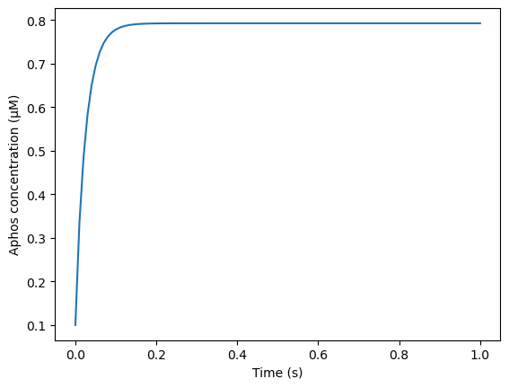
We plot the average Aphos over time.
plt.plot(model_cur.tvec, avg_Aphos)
plt.xlabel('Time (s)')
plt.ylabel('Aphos concentration (μM)')
Text(0, 0.5, 'Aphos concentration (μM)')
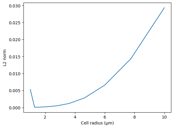
Given the analytical solution at steady state (see below), we can compute the L2 norm of the error.
# L2 error
xvec = d.SpatialCoordinate(cc["Cyto"].dolfin_mesh)
r = d.sqrt(xvec[0]**2 + xvec[1]**2 + (xvec[2])**2)
k_kin = kkin.value
k_p = kp.value
cT = Atot.value
D = Aphos.D
thieleMod = curRadius / np.sqrt(D/k_p)
C1 = k_kin*cT*curRadius**2/((3*D*(np.sqrt(k_p/D)-(1/curRadius)) + k_kin*curRadius)*np.exp(thieleMod) +
                             (3*D*(np.sqrt(k_p/D)+(1/curRadius))-k_kin*curRadius)*np.exp(-thieleMod))
sol = C1*(d.exp(r/np.sqrt(D/k_p))-d.exp(-r/np.sqrt(D/k_p)))/r
L2norm = np.sqrt(d.assemble_mixed((sol-model_cur.sc["Aphos"].u["u"])**2 *dx))
print(f"Current L2 norm is {L2norm}")
ROOT -2026-03-05 07:10:17,300 FFC - WARNING - WARNING: The number of integration points for each cell will be: 1331 (log.py:153)
ROOT -2026-03-05 07:10:17,301 FFC - WARNING - Consider using the option 'quadrature_degree' to reduce the number of points (log.py:153)
Current L2 norm is 0.005309040531563695
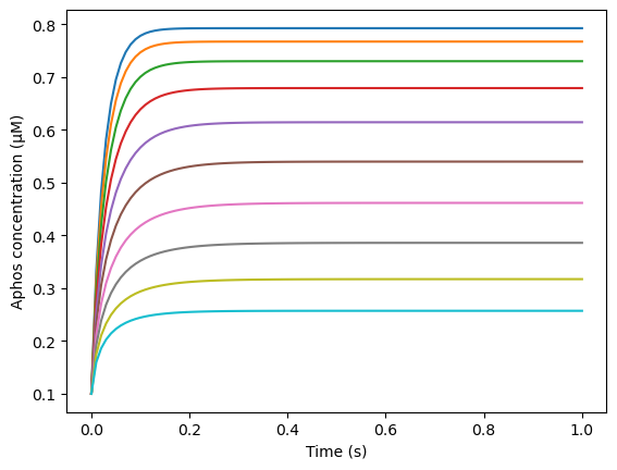
Now we repeat this process for other values of cell radii, to test the dependence of steady state \(A_{phos}\) concentration on cell size
radiusVec = np.logspace(0, 1, num=10)  # currently testing 10 radius values
ss_vec = np.zeros(len(radiusVec))
ss_vec[0] = avg_Aphos[-1]
L2norm_vec = np.zeros(len(radiusVec))
L2norm_vec[0] = L2norm
plt.plot(model_cur.tvec, avg_Aphos)
plt.xlabel('Time (s)')
plt.ylabel('Aphos concentration (μM)')

for i in range(1, len(radiusVec)):
    curRadius = radiusVec[i]
    avg_Aphos = [Aphos.initial_condition]
    pc['VolSA'].value = curRadius/3

    # =============================================================================================
    # Create/load in mesh
    # =============================================================================================
    # Base mesh
    # 0 in second argument corresponds to no inner sphere
    domain, facet_markers, cell_markers = mesh_tools.create_spheres(curRadius, 0, hEdge=0.2)
    # Write mesh and meshfunctions to file
    mesh_folder = pathlib.Path(f"mesh_{curRadius:03f}/")
    mesh_folder.mkdir(exist_ok=True)
    mesh_file = mesh_folder / "DemoSphere.h5"
    mesh_tools.write_mesh(domain, facet_markers, cell_markers, filename=mesh_file)

    # # Define solvers
    parent_mesh = mesh.ParentMesh(
        mesh_filename=f"mesh_{curRadius:03f}/DemoSphere.h5",
        mesh_filetype="hdf5",
        name="parent_mesh",
    )
    config_cur = config.Config()
    model_cur = model.Model(pc, sc, cc, rc, config_cur, parent_mesh)
    config_cur.solver.update(
        {
            "final_t": 1,
            "initial_dt": 0.01,
            "time_precision": 6,
        }
    )

    model_cur.initialize()
    # Write initial condition(s) to file
    results = dict()
    result_folder = pathlib.Path(f"resultsSphere_{i:03d}")
    result_folder.mkdir(exist_ok=True)
    for species_name, species in model_cur.sc.items:
        results[species_name] = d.XDMFFile(
            model_cur.mpi_comm_world, str(result_folder / f"{species_name}.xdmf")
        )
        results[species_name].parameters["flush_output"] = True
        results[species_name].write(model_cur.sc[species_name].u["u"], model_cur.t)

    # save integration measure and volume for computing average Aphos at each time step
    dx = d.Measure("dx", domain=model_cur.cc['Cyto'].dolfin_mesh)
    volume = d.assemble_mixed(1.0*dx)
    # Solve
    while True:
        # Solve the system
        model_cur.monolithic_solve()
        # Save results for post processing
        for species_name, species in model_cur.sc.items:
            results[species_name].write(model_cur.sc[species_name].u["u"], model_cur.t)
        # compute average Aphos concentration at each time step
        int_val = d.assemble_mixed(model_cur.sc['Aphos'].u['u']*dx)
        avg_Aphos.append(int_val / volume)
        # End if we've passed the final time
        if model_cur.t >= model_cur.final_t:
            break

    # store steady state at the end of each run
    ss_vec[i] = avg_Aphos[-1]
    plt.plot(model_cur.tvec, avg_Aphos)

    # compute L2 norm of the error
    xvec = d.SpatialCoordinate(cc["Cyto"].dolfin_mesh)
    r = d.sqrt(xvec[0]**2 + xvec[1]**2 + (xvec[2])**2)
    thieleMod = curRadius / np.sqrt(D/k_p)
    C1 = k_kin*cT*curRadius**2/((3*D*(np.sqrt(k_p/D)-(1/curRadius)) + k_kin*curRadius)*np.exp(thieleMod) +
                                (3*D*(np.sqrt(k_p/D)+(1/curRadius))-k_kin*curRadius)*np.exp(-thieleMod))
    sol = C1*(d.exp(r/np.sqrt(D/k_p))-d.exp(-r/np.sqrt(D/k_p)))/r
    L2norm_vec[i] = d.assemble_mixed((sol-model_cur.sc["Aphos"].u["u"])**2 *dx)

np.savetxt(f"ss_vec.txt", ss_vec)
np.savetxt("L2norm_vec.txt", L2norm_vec)
2026-03-05 07:10:18,373 smart.model - WARNING - Warning! Initial L2-norm of compartment Cyto is 15.817268017258451 (possibly too large). (model.py:1223)
╒════╤═════════════╤══════╤══════════════════╤═════════════╤══════════════╤════════════════╕
│    │ name        │   id │   dimensionality │   num_cells │   num_facets │   num_vertices │
╞════╪═════════════╪══════╪══════════════════╪═════════════╪══════════════╪════════════════╡
│  0 │ parent_mesh │ 3217 │                3 │        4621 │         9926 │           1121 │
├────┼─────────────┼──────┼──────────────────┼─────────────┼──────────────┼────────────────┤
│  1 │ PM          │ 3232 │                2 │        1368 │         2052 │            686 │
├────┼─────────────┼──────┼──────────────────┼─────────────┼──────────────┼────────────────┤
│  2 │ Cyto        │ 3238 │                3 │        4621 │         9926 │           1121 │
╘════╧═════════════╧══════╧══════════════════╧═════════════╧══════════════╧════════════════╛
ROOT -2026-03-05 07:10:26,859 FFC - WARNING - WARNING: The number of integration points for each cell will be: 1331 (log.py:153)
ROOT -2026-03-05 07:10:26,860 FFC - WARNING - Consider using the option 'quadrature_degree' to reduce the number of points (log.py:153)
2026-03-05 07:10:28,219 smart.model - WARNING - Warning! Initial L2-norm of compartment Cyto is 25.747317222491095 (possibly too large). (model.py:1223)
╒════╤═════════════╤══════╤══════════════════╤═════════════╤══════════════╤════════════════╕
│    │ name        │   id │   dimensionality │   num_cells │   num_facets │   num_vertices │
╞════╪═════════════╪══════╪══════════════════╪═════════════╪══════════════╪════════════════╡
│  0 │ parent_mesh │ 6408 │                3 │        8527 │        18254 │           2025 │
├────┼─────────────┼──────┼──────────────────┼─────────────┼──────────────┼────────────────┤
│  1 │ PM          │ 6423 │                2 │        2400 │         3600 │           1202 │
├────┼─────────────┼──────┼──────────────────┼─────────────┼──────────────┼────────────────┤
│  2 │ Cyto        │ 6429 │                3 │        8527 │        18254 │           2025 │
╘════╧═════════════╧══════╧══════════════════╧═════════════╧══════════════╧════════════════╛
ROOT -2026-03-05 07:10:43,439 FFC - WARNING - WARNING: The number of integration points for each cell will be: 1331 (log.py:153)
ROOT -2026-03-05 07:10:43,440 FFC - WARNING - Consider using the option 'quadrature_degree' to reduce the number of points (log.py:153)
2026-03-05 07:10:45,282 smart.model - WARNING - Warning! Initial L2-norm of compartment Cyto is 44.03116950808065 (possibly too large). (model.py:1223)
╒════╤═════════════╤══════╤══════════════════╤═════════════╤══════════════╤════════════════╕
│    │ name        │   id │   dimensionality │   num_cells │   num_facets │   num_vertices │
╞════╪═════════════╪══════╪══════════════════╪═════════════╪══════════════╪════════════════╡
│  0 │ parent_mesh │ 9599 │                3 │       14370 │        30659 │           3349 │
├────┼─────────────┼──────┼──────────────────┼─────────────┼──────────────┼────────────────┤
│  1 │ PM          │ 9614 │                2 │        3838 │         5757 │           1921 │
├────┼─────────────┼──────┼──────────────────┼─────────────┼──────────────┼────────────────┤
│  2 │ Cyto        │ 9620 │                3 │       14370 │        30659 │           3349 │
╘════╧═════════════╧══════╧══════════════════╧═════════════╧══════════════╧════════════════╛
ROOT -2026-03-05 07:11:10,557 FFC - WARNING - WARNING: The number of integration points for each cell will be: 1331 (log.py:153)
ROOT -2026-03-05 07:11:10,558 FFC - WARNING - Consider using the option 'quadrature_degree' to reduce the number of points (log.py:153)
2026-03-05 07:11:13,222 smart.model - WARNING - Warning! Initial L2-norm of compartment Cyto is 73.27959437103064 (possibly too large). (model.py:1223)
╒════╤═════════════╤═══════╤══════════════════╤═════════════╤══════════════╤════════════════╕
│    │ name        │    id │   dimensionality │   num_cells │   num_facets │   num_vertices │
╞════╪═════════════╪═══════╪══════════════════╪═════════════╪══════════════╪════════════════╡
│  0 │ parent_mesh │ 12790 │                3 │       25348 │        53926 │           5797 │
├────┼─────────────┼───────┼──────────────────┼─────────────┼──────────────┼────────────────┤
│  1 │ PM          │ 12805 │                2 │        6460 │         9690 │           3232 │
├────┼─────────────┼───────┼──────────────────┼─────────────┼──────────────┼────────────────┤
│  2 │ Cyto        │ 12811 │                3 │       25348 │        53926 │           5797 │
╘════╧═════════════╧═══════╧══════════════════╧═════════════╧══════════════╧════════════════╛
ROOT -2026-03-05 07:11:58,612 FFC - WARNING - WARNING: The number of integration points for each cell will be: 1331 (log.py:153)
ROOT -2026-03-05 07:11:58,613 FFC - WARNING - Consider using the option 'quadrature_degree' to reduce the number of points (log.py:153)
2026-03-05 07:12:02,682 smart.model - WARNING - Warning! Initial L2-norm of compartment Cyto is 123.42411108388286 (possibly too large). (model.py:1223)
╒════╤═════════════╤═══════╤══════════════════╤═════════════╤══════════════╤════════════════╕
│    │ name        │    id │   dimensionality │   num_cells │   num_facets │   num_vertices │
╞════╪═════════════╪═══════╪══════════════════╪═════════════╪══════════════╪════════════════╡
│  0 │ parent_mesh │ 15981 │                3 │       43865 │        93020 │           9868 │
├────┼─────────────┼───────┼──────────────────┼─────────────┼──────────────┼────────────────┤
│  1 │ PM          │ 15996 │                2 │       10580 │        15870 │           5292 │
├────┼─────────────┼───────┼──────────────────┼─────────────┼──────────────┼────────────────┤
│  2 │ Cyto        │ 16002 │                3 │       43865 │        93020 │           9868 │
╘════╧═════════════╧═══════╧══════════════════╧═════════════╧══════════════╧════════════════╛
ROOT -2026-03-05 07:13:24,343 FFC - WARNING - WARNING: The number of integration points for each cell will be: 1331 (log.py:153)
ROOT -2026-03-05 07:13:24,344 FFC - WARNING - Consider using the option 'quadrature_degree' to reduce the number of points (log.py:153)
2026-03-05 07:13:31,287 smart.model - WARNING - Warning! Initial L2-norm of compartment Cyto is 204.9121277349647 (possibly too large). (model.py:1223)
╒════╤═════════════╤═══════╤══════════════════╤═════════════╤══════════════╤════════════════╕
│    │ name        │    id │   dimensionality │   num_cells │   num_facets │   num_vertices │
╞════╪═════════════╪═══════╪══════════════════╪═════════════╪══════════════╪════════════════╡
│  0 │ parent_mesh │ 19172 │                3 │       76286 │       161500 │          16976 │
├────┼─────────────┼───────┼──────────────────┼─────────────┼──────────────┼────────────────┤
│  1 │ PM          │ 19187 │                2 │       17856 │        26784 │           8930 │
├────┼─────────────┼───────┼──────────────────┼─────────────┼──────────────┼────────────────┤
│  2 │ Cyto        │ 19193 │                3 │       76286 │       161500 │          16976 │
╘════╧═════════════╧═══════╧══════════════════╧═════════════╧══════════════╧════════════════╛
ROOT -2026-03-05 07:16:04,904 FFC - WARNING - WARNING: The number of integration points for each cell will be: 1331 (log.py:153)
ROOT -2026-03-05 07:16:04,905 FFC - WARNING - Consider using the option 'quadrature_degree' to reduce the number of points (log.py:153)
2026-03-05 07:16:16,363 smart.model - WARNING - Warning! Initial L2-norm of compartment Cyto is 341.9112933377822 (possibly too large). (model.py:1223)
╒════╤═════════════╤═══════╤══════════════════╤═════════════╤══════════════╤════════════════╕
│    │ name        │    id │   dimensionality │   num_cells │   num_facets │   num_vertices │
╞════╪═════════════╪═══════╪══════════════════╪═════════════╪══════════════╪════════════════╡
│  0 │ parent_mesh │ 22363 │                3 │      131429 │       277727 │          28937 │
├────┼─────────────┼───────┼──────────────────┼─────────────┼──────────────┼────────────────┤
│  1 │ PM          │ 22378 │                2 │       29738 │        44607 │          14871 │
├────┼─────────────┼───────┼──────────────────┼─────────────┼──────────────┼────────────────┤
│  2 │ Cyto        │ 22384 │                3 │      131429 │       277727 │          28937 │
╘════╧═════════════╧═══════╧══════════════════╧═════════════╧══════════════╧════════════════╛
ROOT -2026-03-05 07:21:17,578 FFC - WARNING - WARNING: The number of integration points for each cell will be: 1331 (log.py:153)
ROOT -2026-03-05 07:21:17,579 FFC - WARNING - Consider using the option 'quadrature_degree' to reduce the number of points (log.py:153)
2026-03-05 07:21:38,265 smart.model - WARNING - Warning! Initial L2-norm of compartment Cyto is 571.1011456970933 (possibly too large). (model.py:1223)
╒════╤═════════════╤═══════╤══════════════════╤═════════════╤══════════════╤════════════════╕
│    │ name        │    id │   dimensionality │   num_cells │   num_facets │   num_vertices │
╞════╪═════════════╪═══════╪══════════════════╪═════════════╪══════════════╪════════════════╡
│  0 │ parent_mesh │ 25554 │                3 │      224553 │       473985 │          49171 │
├────┼─────────────┼───────┼──────────────────┼─────────────┼──────────────┼────────────────┤
│  1 │ PM          │ 25569 │                2 │       49758 │        74637 │          24881 │
├────┼─────────────┼───────┼──────────────────┼─────────────┼──────────────┼────────────────┤
│  2 │ Cyto        │ 25575 │                3 │      224553 │       473985 │          49171 │
╘════╧═════════════╧═══════╧══════════════════╧═════════════╧══════════════╧════════════════╛
ROOT -2026-03-05 07:31:57,945 FFC - WARNING - WARNING: The number of integration points for each cell will be: 1331 (log.py:153)
ROOT -2026-03-05 07:31:57,946 FFC - WARNING - Consider using the option 'quadrature_degree' to reduce the number of points (log.py:153)
2026-03-05 07:32:38,090 smart.model - WARNING - Warning! Initial L2-norm of compartment Cyto is 953.2262987157463 (possibly too large). (model.py:1223)
╒════╤═════════════╤═══════╤══════════════════╤═════════════╤══════════════╤════════════════╕
│    │ name        │    id │   dimensionality │   num_cells │   num_facets │   num_vertices │
╞════╪═════════════╪═══════╪══════════════════╪═════════════╪══════════════╪════════════════╡
│  0 │ parent_mesh │ 28745 │                3 │      383722 │       808913 │          83405 │
├────┼─────────────┼───────┼──────────────────┼─────────────┼──────────────┼────────────────┤
│  1 │ PM          │ 28760 │                2 │       82938 │       124407 │          41471 │
├────┼─────────────┼───────┼──────────────────┼─────────────┼──────────────┼────────────────┤
│  2 │ Cyto        │ 28766 │                3 │      383722 │       808913 │          83405 │
╘════╧═════════════╧═══════╧══════════════════╧═════════════╧══════════════╧════════════════╛
ROOT -2026-03-05 08:17:52,813 FFC - WARNING - WARNING: The number of integration points for each cell will be: 1331 (log.py:153)
ROOT -2026-03-05 08:17:52,814 FFC - WARNING - Consider using the option 'quadrature_degree' to reduce the number of points (log.py:153)
Compare model results to analytical solution and previous results#
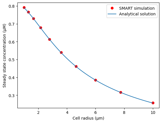
Here, we plot the steady-state concentration as a function of cell radius, according to the analytical solution and the SMART numerical solution. The analytical solution for the average concentration in the cytosol at steady state is given in Meyers and Odde 2006 and is included here for ease of reference:
The full spatial dependence (used to compute the L2 norm of the error) is expressed as: $\( c_A = 2 C_1 \frac{\sinh(r/L_{gradient})}{r}\\ \)$
where \(r\) is the distance from the center of the sphere.
plt.plot(radiusVec, ss_vec, 'ro')
radiusTest = np.logspace(0, 1, 100)
thieleMod = radiusTest / np.sqrt(D/k_p)
C1 = k_kin*cT*radiusTest**2/((3*D*(np.sqrt(k_p/D)-(1/radiusTest)) + k_kin*radiusTest)*np.exp(thieleMod) +
                             (3*D*(np.sqrt(k_p/D)+(1/radiusTest))-k_kin*radiusTest)*np.exp(-thieleMod))
cA = (6*C1/radiusTest)*(np.cosh(thieleMod)/thieleMod - np.sinh(thieleMod)/thieleMod**2)
plt.plot(radiusTest, cA)
plt.xlabel("Cell radius (μm)")
plt.ylabel("Steady state concentration (μM)")
plt.legend(("SMART simulation", "Analytical solution"))
<matplotlib.legend.Legend at 0x7f323c30a9b0>
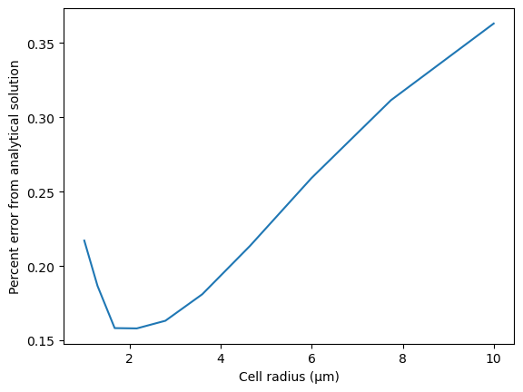
We compare the SMART results to the analytical solution, requiring that the steady state concentration in simulations deviates less than 1% from the known analytical value.
# quantify percent error
thieleMod = radiusVec / np.sqrt(D/k_p)
C1 = k_kin*cT*radiusVec**2/((3*D*(np.sqrt(k_p/D)-(1/radiusVec)) + k_kin*radiusVec)*np.exp(thieleMod) +
                            (3*D*(np.sqrt(k_p/D)+(1/radiusVec))-k_kin*radiusVec)*np.exp(-thieleMod))
cA = (6*C1/radiusVec)*(np.cosh(thieleMod)/thieleMod - np.sinh(thieleMod)/thieleMod**2)
percentError = 100*np.abs(ss_vec - cA) / cA
plt.plot(radiusVec, percentError)
plt.xlabel("Cell radius (μm)")
plt.ylabel("Percent error from analytical solution")
assert all(percentError <
           1), f"Example 2 results deviate {max(percentError):.3f}% from the analytical solution"
rmse = np.sqrt(np.mean(percentError**2))
print(f"RMSE with respect to analytical solution = {rmse:.3f}%")
RMSE with respect to analytical solution = 0.231%
As a regression test, we compare the steady-state values from this SMART simulation with stored values run in a previous version of SMART. We require that the results deviate less than 0.01% from the stored values.
# check that solution is not too far from previous numerical solution (regression test)
ss_vec_ref = np.array([0.79232888, 0.76696666, 0.72982203, 0.67888582, 0.61424132,
                       0.53967824, 0.46147368, 0.38586242, 0.31707563, 0.25709714])
percentErrorRegression = 100*np.abs(ss_vec - ss_vec_ref) / ss_vec_ref
assert all(percentErrorRegression <
           0.01), f"Failed regression test: Example 3 results deviate {max(percentErrorRegression):.3f}% from the previous numerical solution"
rmse_regression = np.sqrt(np.mean(percentErrorRegression**2))
print(f"RMSE with respect to previous numerical solution = {rmse_regression:.3f}%")
RMSE with respect to previous numerical solution = 0.000%
Plot L2 norm of the error at different cell radii.
plt.plot(radiusVec, L2norm_vec)
plt.xlabel("Cell radius (μm)")
plt.ylabel("L2 norm")
Text(0, 0.5, 'L2 norm')